SINUMERIK 840D sl/828D. Job Planning. Programming Manual (2010-2018) - page 23
Motion synchronous actions
10.4 Actions in synchronized actions
10.4.22
Leading value coupling (LEADON, LEADOF)
Note
This function is not available for SINUMERIK 828D!
Function
The axial leading value coupling can be programmed in synchronized actions without
restriction. The changing of a curve table for an existing coupling without a previous
resynchronization is optionally possible only in synchronized actions.
Syntax
Activate master value coupling
DO LEADON (following axis, leading axis, curve table no., OVW)
Deactivate leading value coupling
DO LEADOF(following axis, leading axis, leading axis 2)
Significance
Activate axial leading value coupling:
...DO LEADON(FA, LA, NR, OVW) with:
FA: Following axis
LA: Leading axis
NR: Number of the stored curve table
OVW: Permit overwriting an existing coupling with changed
curve table
Deactivate axial leading value coupling:
...DO LEADOF(FA, LA)
with:
FA: Following axis
LA: Leading axis, optional
... DO LEADOF(FA)
Shortened form without specification of leading axis
Job Planning
Programming Manual, 03/2010, 6FC5398-2BP20-1BA0
613
Motion synchronous actions
10.4 Actions in synchronized actions
Activate access with synchronized actions RELEASE
The axis to be coupled is released for synchronized action access by invoking the RELEASE
function for the axis.
Example:
RELEASE (XKAN)
ID=1 every SR1==1 to LEADON(CACH,XKAN,1)
OVW=0 (default value)
Without a resynchronization, no new curve table can be specified for an existing coupling. A
change of the curve table requires the previous deactivation of the existing coupling and a
reactivation with the changed curve table number. This causes a resynchronization of the
coupling.
Changing the curve table for an existing coupling using OVW=1
OVW=1 can be used to specify a new curve table to an existing coupling. No resynchronization
is performed. The following axis attempts as fast as possible to follow the position values
specified by the new curve table.
Example of on-the-fly parting
An extruded material which passes continuously through the operating area of a cutting tool
must be cut into parts of equal length.
X axis: Axis in which the extruded material moves, WCS
X1 axis: Machine axis of extruded material, MCS
Y axis: Axis in which cutting tool "tracks" the extruded material
It is assumed that the infeed and control of the cutting tool are controlled via the PLC. The
signals at the PLC interface can be evaluated to determine whether the extruded material
and cutting tool are synchronized.
Actions
Activate coupling, LEADON
Deactivate coupling, LEADOF
Set actual values, PRESETON
Job Planning
614
Programming Manual, 03/2010, 6FC5398-2BP20-1BA0
Motion synchronous actions
10.4 Actions in synchronized actions
Program code
Comments
N100 R3=1500
; Length of a part to be
cut off
N200 R2=100000 R13=R2/300
N300 R4=100000
N400 R6=30
; Start position Y axis
N500 R1=1
; Start condition for
conveyor axis
N600 LEADOF(Y,X)
; Delete any existing
coupling
N700 CTABDEF(Y,X,1,0)
; Table definition
N800 X=30 Y=30
; Value pairs
N900 X=R13 Y=R13
N1000 X=2*R13 Y=30
N1100 CTABEND
; End of table
definition
N1200 PRESETON(X1,0)
; PRESET at beginning
N1300 Y=R6 G0
; Start position Y axis,
axis is linear
N1400 ID=1 WHENEVER $AA_IW[X]>$R3 DO PESETON(X1,0)
; PRESET after length
R3, new start after
disconnecting
N1500 RELEASE(Y)
N1800 ID=6 EVERY $AA_IM[X]<10 DO LEADON(Y,X,1)
; For X < 10, couple Y
to X via table 1
N1900 ID=10 EVERY $AA_IM[X]>$R3-30 DO EADOF(Y,X)
; > 30 before traversed
parting distance,
deactivate coupling
N2000 WAITP(X)
N2100 ID=7 WHEN $R1==1 DO MOV[X]=1 FA[X]=$R4
; Set extruded material
axis continuously in
motion
N2200 M30
Job Planning
Programming Manual, 03/2010, 6FC5398-2BP20-1BA0
615
Motion synchronous actions
10.4 Actions in synchronized actions
10.4.23
Measuring (MEAWA, MEAC)
Function
Compared with use in traverse blocks of the part program, the measuring function can be
activated and deactivated as required.
For further information concerning measuring, see special motion commands "Extended
measuring function"
Syntax
Axial measurement without deletion of distance-to-go
MEAWA[axis]=(mode, trigger_event_1, ..._4)
Continuous measurement without deleting distance-to-go
MEAC[axis]=(mode, measurement_memory, trigger_event_1, ..._4)
Significance
Program code
Comments
DO MEAWA
; Switch-in axial measurement
DO MEAC
; Switch-in continuous
measurement
Axis
; The name of the axis for
which measurement is taken
Mode
; Specification of the tens
Specification of the units
decade
decade
0: active measuring system
0: Cancel measuring job
Number of the measuring
up to 4 trigger events can be
systems (depending on the
activated
mode)
1: concurrently
1: 1st measuring system
2: successively
2: 2nd measuring system
3: as for 2, however no
3: both measuring systems
monitoring of trigger event1 at
the start
Trigger_event_1
;
: rising edge, probe
to
-1: falling edge, probe 1
trigger_event_4
optional
2: rising edge, probe 2
optional
-2: falling edge, probe 2
optional
Measurement
; Number of the FIFO
memory
circulating storage
Job Planning
616
Programming Manual, 03/2010, 6FC5398-2BP20-1BA0
Motion synchronous actions
10.4 Actions in synchronized actions
10.4.24
Initialization of array variables (SET, REP)
Function
Array variables can be initialized or described with particular values in synchronized actions.
Note
Only variables that can be described in synchronized actions are possible. Machine data
cannot therefore be initialized. Axis variables cannot be specified using the NO_AXIS value.
Syntax
DO ARRAY[n,m]=SET(<value1>,<value2>,...)
DO ARRAY[n,m]=REP(<value>)
Significance
ARRAY[n,m]
Programmed array indices set
Initialization starts at the programmed array indexes.
For 2D arrays, the second index is incremented first.
This is not done with axis indices.
SET(<value1>,<value2>,...)
Initialization with value lists
The array is described from the programmed array
indices onwards using the SET parameters. As many
array elements are assigned as values are
programmed. If more values than exist in the remaining
array elements are programmed, an alarm is triggered.
REP(<value>)
Initialization with the same values
The array is described from the programmed array
indices to the end of the array and repeated using the
parameter <value>) of REP.
Example
Program code
Comments
WHEN TRUE DO SYG_IS[0]=REP(0)
;
Result:
WHEN TRUE DO SYG_IS[1]=SET(3,4,5)
; SYG_IS[0]=0
SYG_IS[1]=3
SYG_IS[2]=4
SYG_IS[3]=5
SYG_IS[4]=0
Job Planning
Programming Manual, 03/2010, 6FC5398-2BP20-1BA0
617
Motion synchronous actions
10.4 Actions in synchronized actions
10.4.25
Set/delete wait markers (SETM, CLEARM)
Function
Wait markers can be set or deleted in synchronized actions in order to e.g. coordinate
channels with one another.
Syntax
DO SETM(<marker number>)
DO CLEARM(<marker number>)
Significance
SETM
Command to set the wait marker for the channel
The command SETM can be programmed in the part program
and in the action component of a synchronized action. It sets
the marker (<marker number>) for the channel in which the
command is applied.
CLEARM
Command to delete the wait marker for the channel
The command CLEARM can be programmed in the part program
and in the action component of a synchronized action. It
deletes the marker (<marker number>) for the channel in which
the command is applied.
<marker number>
Wait marker
Job Planning
618
Programming Manual, 03/2010, 6FC5398-2BP20-1BA0
Motion synchronous actions
10.4 Actions in synchronized actions
10.4.26
Fault responses (SETAL)
Function
Fault responses can be programmed using synchronized actions. Status variables are
interrogated and the corresponding actions initiated.
Some possible responses to error conditions are:
● Stop axis (override=0)
● Set alarm
SETAL can set cycle alarms from synchronized actions.
● Set output
● All possible actions in synchronized actions
Syntax
Set cycle alarm:
DO SETAL(<alarm number>)
Significance
SETAL
Command to set a cycle alarm
<alarm number>
Alarm number
Cycle alarm range for users:
65000 ... 69999
Example
Program code
Comments
ID=67 WHENEVER ($AA_IM[X1]-$AA_IM[X2])<4.567 DO $AA_OVR[X2]=0
; Stop axis X2 if the safety
clearance between axes X1
and X2 is too small.
ID=67 WHENEVER ($AA_IM[X1]-$AA_IM[X2])<4.567 DO SETAL(65000)
; Set alarm 65000 if the
safety clearance between
axes X1 and X2 is too
small.
Job Planning
Programming Manual, 03/2010, 6FC5398-2BP20-1BA0
619
Motion synchronous actions
10.4 Actions in synchronized actions
10.4.27
Travel to fixed stop (FXS, FXST, FXSW, FOCON, FOCOF)
Function
The commands for the function "travel to fixed stop" are programmed using the part program
commands FXS, FXST and FXSW in synchronized actions/technology cycles.
Activation can take place without movement, the torque is immediately limited. As soon as
the axis is moved via a setpoint, the limit stop monitor is activated.
Travel with limited torque/force (FOC)
The function allows torque/force to be changed any time via synchronized actions and can
be modally activated or block-for-block.
Syntax
FXS[<axis>]
FXST[<axis>]
FXSW[<axis>]
FOCON[<axis>]
FOCOF[<axis>]
Significance
FXS
Can only be selected in systems with digital drives (FDD, MSD, HLA)
FXST
Changes the clamping torque FXST
FXSW
Changes the monitoring window FXSW
FOCON
Activates the modally effective torque/force limiting
FOCOF
Disables the torque/force limiting
<axis>
Axis identifier
The following is permissible:
• Geometry axis identifier
• Channel axis identifier
• Machine axis identifier
Note
A selection may only be carried out once.
Job Planning
620
Programming Manual, 03/2010, 6FC5398-2BP20-1BA0
Motion synchronous actions
10.4 Actions in synchronized actions
Examples
Example 1: Travel to fixed stop (FXS), initiated using a synchronized action
Program code
Comments
Y axis:
; Static synchronized actions
Activate:
N10 IDS=1 WHENEVER (($R1==1) AND $AA_FXS[y]==0)) D $R1=0 FXS[Y]=1 FXST[Y]=10 FA[Y]=200 POS[Y]=150
; FXS is activated for axis Y by setting
$R1=1, the effective torque is reduced
to 10% and travel is started towards the
fixed stop.
N11 IDS=2 WHENEVER ($AA_FXS[Y]==4) DO FXST[Y]=30
; As soon as the fixed stop was detected
($AA_FXS[Y]==4), the torque was reduced
to 30%.
N12 IDS=3 WHENEVER ($AA_FXS[Y]==1) DO FXST[Y]=$R0
; After the fixed stop is reached the
torque is controlled depending on R0.
N13 IDS=4 WHENEVER (($R3==1) AND $AA_FXS[Y]==1)) DO FXS[Y]=0 FA[Y]=1000 POS[Y]=0
; De-selection depending on R3 and
retract.
N20 FXS[Y]=0 G0 G90 X0 Y0
; Normal program execution:
N30 RELEASE(Y)
; Release axis Y for motion in the
synchronized action.
N40 G1 F1000 X100
; Motion of another axis.
N50 ...
N60 GET(Y)
; Include axis Y back into the path group
Example 2: Activating torque/force limiting (FOC)
Program code
Comments
N10 FOCON[X]
; Modal activation of limiting.
N20 X100 Y200 FXST[X]=15
; X travels with reduced torque (15%).
N30 FXST[X]=75 X20
; The torque is changed to 75%, X travels with
this limited torque.
N40 FOCOF[X]
; The torque limiting is switched-out.
Job Planning
Programming Manual, 03/2010, 6FC5398-2BP20-1BA0
621
Motion synchronous actions
10.4 Actions in synchronized actions
Further Information
Multiple selection
If the function is called once more due to incorrect programming after activating (FXS[axis] =
1)) the following alarm is output:
Alarm 20092 "Travel to fixed stop is still active"
Programming, that either interrogates $AA_FXS[ ] or a dedicated bit memory (here R1) in the
condition, avoids activating the function "Part program fragment" a multiple number of times:
Program code
N10 R1=0
N20 IDS=1 WHENEVER ($R1==0 AND
$AA_IW[AX3] > 7) DO R1=1 FXST[AX1]=12
Block-related synchronized actions
By programming a block-related synchronized action, travel to fixed stop can be connected
during an approach motion.
Example:
Program code
Comments
N10 G0 G90 X0 Y0
N20 WHEN $AA_IW[X] > 17 DO FXS[X]=1
; FXS is activated if X reaches a
position greater than 17 mm.
N30 G1 F200 X100 Y110
Static and block-related synchronized actions
In static and block-related synchronized actions, the same commands FXS, FXST and FXSW can
be used as in a normal part program execution. The values assigned can be resulted from a
calculation.
Job Planning
622
Programming Manual, 03/2010, 6FC5398-2BP20-1BA0
Motion synchronous actions
10.4 Actions in synchronized actions
10.4.28
Determining the path tangent in synchronized actions
Function
The system variable $AC_TANEB (Tangent ANgle at End of Block), which can be read in
synchronized actions, calculates the angle between the path tangent at the end of the
current block and the path tangent at the start of the programmed following block.
Parameters
The tangent angle is always output positive in the range 0.0 to 180.0 degrees. If there is no
following block in the main run, the angle -180.0 degrees is output.
The system variable $AC_TANEB should not be read for blocks generated by the system
(intermediate blocks). The system variable $AC_BLOCKTYPE is used to tell whether it is a
programmed block (main block).
Example
ID=2 EVERY $AC_BLOCKTYPE==0 DO $SR1 = $AC_TANEB
10.4.29
Determining the current override
Function
The current override
(NC component) can be read and written with system variables:
$AA_OVR Axial override
$AC_OVR Path override
in synchronized actions.
The override defined by the PLC is provided for synchronized actions to read in the system
variables:
$AA_PLC_OVR Axial override
$AC_PLC_OVR Path override
The resulting override
is provided for synchronized actions to read in the system variables:
$AA_TOTAL_OVR Axial override
$AC_TOTAL_OVR Path override
The resulting override can be calculated as:
$AA_OVR * $AA_PLC_OVR or
$AC_OVR * $AC_PLC_OVR
Job Planning
Programming Manual, 03/2010, 6FC5398-2BP20-1BA0
623
Motion synchronous actions
10.4 Actions in synchronized actions
10.4.30
Time use evaluation of synchronized actions
Function
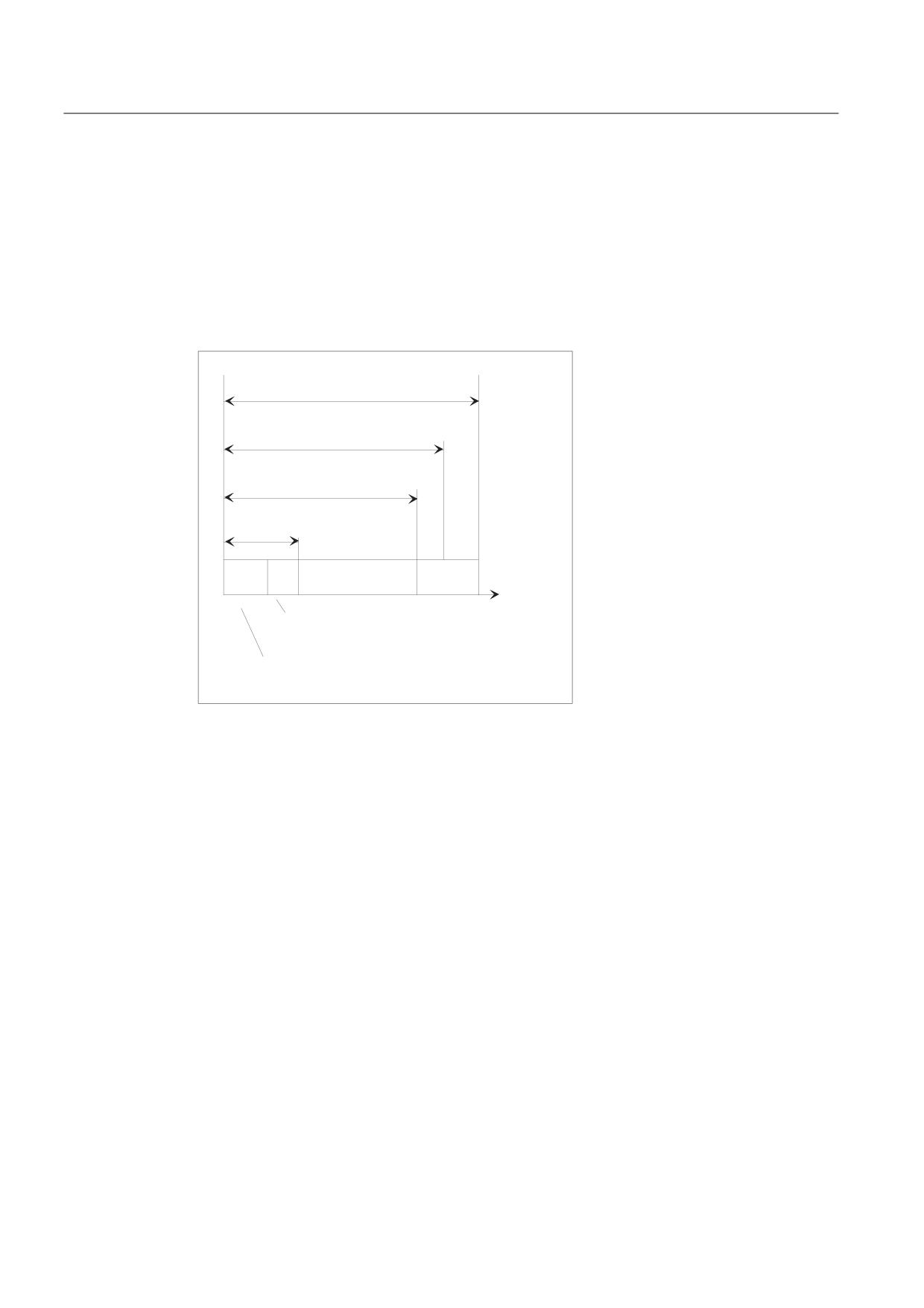
In a interpolation cycle, synchronized actions have to be both interpreted and motions
calculated by the NC. The system variables presented below provide synchronized actions
with information about the current time shares that synchronized actions have of the
interpolation cycle and about the computation time of the position controllers.
,32 F\FOH
01B,32B0$;B/2$'
/LPLWLQJ YDOXH IRU ,32 F\FOH XWLOL]DWLRQ
$1B,32B$&7B/2$'
&XUU ,32 FRPSXWLQJ WLPH LQFO FKDQQHO V\QF
K
$1B6<1&B$&7B/2$'
&XUUHQW FRPS WLPH IRU 6$
IRU DOO FKDQQHOV
W
$&B6<1&B$&7B/2$'
FKDQQHOb
&RPS WLPH IRU V\QFK DFWLRQV RQ FKDQQHO
$&B6<1&B$&7B/2$'
FKDQQHOb
&RPS WLPH IRU V\QFK DFWLRQV RQ FKDQQHO
Significance
The variables only have valid values if machine data $MN_IPO_MAX_LOAD is greater than 0.
Otherwise the variables for both SINUMERIK powerline and solution line systems always
specify the net computing time during which the interrupts caused by HMI are no longer
taken into account. The net computing time results from:
● synchronized action time,
● position control time and
● remaining IPO computing time without interrupts caused by HMI
Job Planning
624
Programming Manual, 03/2010, 6FC5398-2BP20-1BA0
Motion synchronous actions
10.4 Actions in synchronized actions
The system variables always contain the values of the previous IPO cycle.
$AN_IPO_ACT_LOAD
current IPO computing time (incl. synchronized actions of all
channels)
$AN_IPO_MAX_LOAD
longest IPO computing time (incl. synchronized actions of all
channels)
$AN_IPO_MIN_LOAD
shortest IPO computing time (incl. synchronized actions of all
channels)
$AN_IPO_LOAD_PERCENT current IPO computing time as percentage of IPO cycle (%)
$AN_SYNC_ACT_LOAD
current computing time for synchronized actions over all channels
$AN_SYNC_MAX_LOAD
longest computing time for synchronized actions over all channels
$AN_SYNC_TO_IPO
percentage share that the synchronized actions have of the
complete IPO computer time (over all channels)
$AC_SYNC_ACT_LOAD
current computing time for synchronized actions in the channel
$AC_SYNC_MAX_LOAD
longest computing time for synchronized actions in the channel
$AC_SYNC_AVERAGE_LOAD average computing time for synchronized actions in the channel
$AN_SERVO_ACT_LOAD
current computing time of the position controller
$AN_SERVO_MAX_LOAD
longest computing time of the position controller
$AN_SERVO_MIN_LOAD
shortest computing time of the position controller
Variable for the overload notification:
The machine data $MN_IPO_MAX_LOAD is used to set the net IPO computing time
(as % of IPO cycle) from which the system variable
$AN_IPO_LOAD_LIMIT will be set to TRUE. If the current load falls below this limit, the variable
is again set to FALSE. If the machine data is 0, the entire diagnostic function is deactivated.
The evaluation of $AN_IPO_LOAD_LIMIT allows the user to define a strategy for avoiding a level
overflow.
Job Planning
Programming Manual, 03/2010, 6FC5398-2BP20-1BA0
625
Motion synchronous actions
10.5 Technology cycles
10.5
Technology cycles
Function
As an action in synchronized actions, you can invoke programs. These must consist only of
functions that are permissible as actions in synchronized actions. Programs structured in this
way are called technology cycles.
Technology cycles are stored in the control as subprograms.
It is possible to process several technology cycles or actions in parallel in one channel.
Programming
The following rules apply when programming technology cycles:
● End of program is programmed with M02/M17/M30/RET.
● All actions specified in ICYCOF can be processed in one cycle without waiting cycles within
one program level.
● Up to 8 technology cycles can be queried one after another per synchronized action.
● Technology cycles are also possible in synchronized actions that are effective block-for-
block (non-modal).
● Both IF check structures and GOTO, GOTOF and GOTOB jump instructions can be
programmed.
● The following applies to blocks with DEF and DEFINE instructions:
- DEF and DEFINE instructions are read over (ignored) into technology cycles.
- These result in alarm messages if the syntax is incorrect or incomplete.
- They can be read over without an alarm message without being set-up themselves.
- They are taken into full consideration with value assignments as part program cycle.
Parameter transfer
Parameter transfer to technology cycles is possible. Both simple data types which are
transferred as formal "Call by Value" parameters and default settings which take effect when
technology cycles are called up are taken into account. These are:
● Programmed default values when no transfer parameters are programmed.
● Standard parameter with initial values.
● Non-initialized actual parameters with a default value are transferred.
Job Planning
626
Programming Manual, 03/2010, 6FC5398-2BP20-1BA0
Motion synchronous actions
10.5 Technology cycles
Sequence
Technology cycles are started as soon as their conditions have been fulfilled. Each line in a
technology cycle is processed in a separate IPO cycle. Several IPO cycles are required to
execute positioning axes. Other functions are executed in one cycle. Blocks are sequentially
executed in the technology cycle.
If actions that are mutually exclusive are called up in the same interpolation cycle, the action
that is called up from the synchronized action with the higher ID number becomes active.
Examples
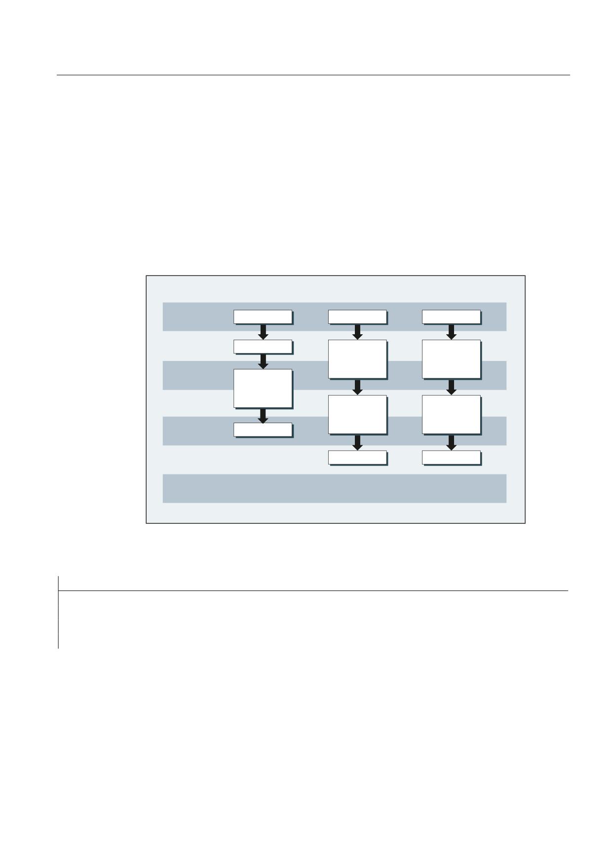
Example 1: Axis programs are started by setting digital inputs
,'
,'
,'
,32 F\FOH
&RQGLWLRQ
&RQGLWLRQ
&RQGLWLRQ
,32 F\FOH
0
326 ><@
326 >=@
,32 F\FOH
326 >;@
,32 F\FOH
326 ><@
326 >=@
,32 F\FOH
0
,32 F\FOH
0
0
,32 F\FOH
Main program:
Program code
Comments
ID=1 EVERY $A_IN[1]==1 DO AXIS_X
; If input 1 is 1, start axis program AXIS_X.
ID=2 EVERY $A_IN[2]==1 DO AXIS_Y
; If input 2 is 1, start axis program AXIS_Y.
ID=3 EVERY $A_IN[3]==1 DO AXIS_Z
; If input 3 is 1, start axis program AXIS_Z.
M30
Axis program AXIS_X:
Program code
M100
POS[X]=100 FA[X]=300
M17
Job Planning
Programming Manual, 03/2010, 6FC5398-2BP20-1BA0
627
Motion synchronous actions
10.5 Technology cycles
Axis program AXIS_Y:
Program code
POS[Y]=10 FA[Y]=200
POS[Y]=-10
M17
Axis program AXIS_Z:
Program code
POS[Z]=90 FA[Z]=250
POS[Z]=-90
M17
Example 2: Various program sequences in the technology cycle
Program code
PROC CYCLE
N10 DEF REAL VALUE=12.3
N15 DEFINE ABC AS G01
Both blocks are read over without the variables and/or macros being set-up.
Program code
PROC CYCLE
N10 DEF REAL
N15 DEFINE ABC G01
Both blocks still generate the NC alarm because the syntax is not written correctly.
Program code
PROC CYCLE
N10 DEF AXIS AXIS1=XX2
If axis XX2 is not known, alarm 12080 is output. Otherwise the block is read over without
alarms and without the variables being set up.
Program code
PROC CYCLE
N10 DEF AXIS AXIS1
N15 G01 X100 F1000
N20 DEF REAL VALUE1
Block N20 always generates alarm 14500, since a definition operation is not permitted after
the 1st program command.
Job Planning
628
Programming Manual, 03/2010, 6FC5398-2BP20-1BA0
Motion synchronous actions
10.5 Technology cycles
10.5.1
Context variable ($P_TECCYCLE)
Function
The $P_TECCYCLE variables can be used to divide programs into synchronized action
programs and preprocessing programs. It is then possible to process blocks or program
sequences that are written correctly (in terms of syntax) or alternatively process them as the
part program cycle.
Interpreting context variable
The $P_TECCYCLE system variable allows context-specific interpretation of program
sections to be controlled in technology cycles:
IF $P_TECCYCLE==TRUE
; Program sequence for technology cycle in synchronized
action
ELSE
; Program sequence for part program cycle
ENDIF
Note
A block with incorrect or unauthorized program syntax as well as unknown value
assignments also result in an alarm message in the part program cycle.
Example
Program sequence with interrogation of $P_TECCYCLE in the technology cycle:
Program code
Comments
PROC CYCLE
N10 DEF REAL VALUE1
; Is read over in the technology cycle.
N15 G01 X100 F1000
N20 IF $P_TECCYCLE==TRUE
; Program sequence for technology cycle (without variable VALUE1)
N30 ELSE
; Program sequence for part program cycle (variable VALUE1 is
available)
N40 ENDIF
Job Planning
Programming Manual, 03/2010, 6FC5398-2BP20-1BA0
629
Motion synchronous actions
10.5 Technology cycles
10.5.2
Call-by-value parameters
Function
Technology cycles can be defined using call-by-value parameters. Simple data types such
as INT, REAL, CHAR, STRING, AXIS and BOOL can be used as parameters.
Note
Formal parameters that are transferred as call-by-value cannot be arrays.
Actual parameters can also comprise default parameters (see "Default parameter
initialization (Page 630)").
Syntax
ID=1 WHEN $AA_IW[X]>50 DO TEC(IVAL,RVAL,,SVAL,AVAL)
A default value is transferred for non-initialized actual parameters:
ID=1 WHEN $AA_IW[X]>50 DO TEC(IVAL,RVAL,,SYG_SS[0],AVAL)
10.5.3
Default parameter initialization
Function
Default parameters can also be provided with an initial value in the PROC instructions.
Syntax
Assign default parameters in the technology cycle:
PROC TEC (INT IVAL=1, REAL RVAL=1.0, CHAR CVAL='A', STRING[10] SVAL="ABC", AXIS
AVAL=X, BOOL BVAL=TRUE)
If a current parameter consists of a default parameter, the initial value is transferred from the
PROC instruction. This applies both in the part program and in synchronized actions.
Example
Program code
Comments
TEC (IVAL, RVAL, SVAL, AVAL)
;
For CVAL and BVAL, the initial value applies
Job Planning
630
Programming Manual, 03/2010, 6FC5398-2BP20-1BA0
Motion synchronous actions
10.5 Technology cycles
10.5.4
Control processing of technology cycles (ICYCOF, ICYCON)
Function
The ICYCOF and ICYCON language commands are used to control the time processing of
technology cycles.
All blocks of a technology cycle are processed in just one interpolation cycle using ICYCOF.
All actions which require several cycles result in parallel processes with ICYCOF.
Application
With ICYCON, command axis movements can result in a delay to the processing of a
technology cycle. If this is not wanted, then all actions can be processed with ICYCOF in one
interpolation cycle without waiting times.
Syntax
The following applies to the cyclic processing of technology cycles:
ICYCON each block of a technology cycle is processed in a separate IPO cycle following
ICYCON.
ICYCOF all subsequent blocks of a technology cycle are processed in one interpolation cycle
following ICYCOF.
Note
The two ICYCON and ICYCOF language commands are only effective within the program
level. Both commands are easily overlooked without a response in the part program.
Example of ICYCOF processing mode
Program code
Comments
IPO cycle
; PROC TECHNOCYC
1.
; $R1=1
2.25
; POS[X]=100
26.
; ICYCOF
26.
; $R1=2
26.
; $R2=$R1+1
26.
; POS[X]=110
26.
; $R3=3
26.
; RET
Job Planning
Programming Manual, 03/2010, 6FC5398-2BP20-1BA0
631
Motion synchronous actions
10.5 Technology cycles
10.5.5
Cascading technology cycles
Function
Up to 8 technology cycles can be processed switched in line. Several technology cycles can
then be programmed in one synchronized action.
Syntax
ID=1 WHEN $AA_IW[X]>50 DO TEC1($R1) TEC2 TEC3(X)
Sequence of execution
The technology cycles are processed in order (in a cascade) working from left to right in
accordance with the aforementioned programming. If a cycle is to be processed in ICYCON
mode, this delays all the subsequent processing actions. An alarm aborts all subsequent
actions.
10.5.6
Technology cycles in non-modal synchronized actions
Function
Technology cycles are also possible in non-modal synchronized actions.
If the processing time of a technology cycle is longer than the processing time of the
associated block, the technology cycle is aborted when the block is changed.
Note
A technology cycle does not prevent the block change.
10.5.7
Check structures (IF)
Function
IF check structures can be used in synchronized actions for branches in the processing
sequence of technology cycles.
Syntax
IF <condition>
$R1=1
[ELSE] optional
$R1=0
ENDIF
Job Planning
632
Programming Manual, 03/2010, 6FC5398-2BP20-1BA0
Motion synchronous actions
10.5 Technology cycles
10.5.8
Jump instructions (GOTO, GOTOF, GOTOB)
Function
Jump instructions (GOTO, GOTOF, GOTOB) are possible in technology cycles. The
specified labels must be present in the subprograms to prevent alarms from being triggered.
Note
Labels and block numbers may only be constants.
Syntax
Unconditional jumps
GOTO Label, block number
GOTOF Label, block number
GOTOB Label, block number
Jump instructions and jump destinations
GOTO
Firstly jump forwards and then backwards
GOTOF
Jump forwards
GOTOB
Jump backwards
Label:
Jump marker
Block number
Jump destination for this block
N100
Block number is subblock
:100
Block number is main block
Job Planning
Programming Manual, 03/2010, 6FC5398-2BP20-1BA0
633
Motion synchronous actions
10.5 Technology cycles
10.5.9
Lock, unlock, reset (LOCK, UNLOCK, RESET)
Function
The sequence of a technology cycle can be locked, unlocked or reset using another modal
synchronized action.
Syntax
LOCK(<n1>,<n2>,...)
UNLOCK(<n1>,<n2>,...)
RESET(<n1>,<n2>,...)
Significance
LOCK
Command to lock synchronized actions
The active action is interrupted.
UNLOCK
Command to unlock synchronized actions
RESET
Command to reset technology cycles
<n1>,<n2>,...
Identification numbers of synchronized actions or technology cycles
that are to be locked, unlocked or reset.
Interlocking synchronized actions
Modal synchronized actions with ID numbers <n> = 1 ... 64 can be interlocked from the PLC.
The associated condition is no longer evaluated and execution of the associated function is
locked in the NCK.
All synchronized actions can be locked indiscriminately with one signal in the PLC interface.
Note
A programmed synchronized action is active as standard and can be protected against
overwriting/locking by a machine data setting.
It should not be possible for end users to modify synchronized actions defined by the
machine manufacturer.
Job Planning
634
Programming Manual, 03/2010, 6FC5398-2BP20-1BA0
Motion synchronous actions
10.5 Technology cycles
Examples
Example 1: Lock synchronized actions (LOCK)
Program code
N100 ID=1 WHENEVER $A_IN[1]==1 DO M130
N200 ID=2 WHENEVER $A_IN[2]==1 DO LOCK(1)
Example 2: Unlock synchronized actions (UNLOCK)
Program code
N100 ID=1 WHENEVER $A_IN[1]==1 DO M130
N200 ID=2 WHENEVER $A_IN[2]==1 DO LOCK(1)
N250 ID=3 WHENEVER $A_IN[3]==1 DO UNLOCK(1)
Example 3: Interrupt technology cycle (RESET)
Program code
N100 ID=1 WHENEVER $A_IN[1]==1 DO M130
N200 ID=2 WHENEVER $A_IN[2]==1 DO RESET(1)
Job Planning
Programming Manual, 03/2010, 6FC5398-2BP20-1BA0
635
Motion synchronous actions
10.6 Delete synchronized action (CANCEL)
10.6
Delete synchronized action (CANCEL)
Function
The CANCEL command can be used to cancel (delete) a modal or a static synchronized action
from the part program.
If a synchronized action is canceled while the positioning axis movement that was activated
from it is still active, the positioning axis movement is interrupted. If this is not desirable, axis
motion can be braked with deletion of the axial distance-to-go before the CANCEL command.
Syntax
CANCEL(<n1>,<n2>,...)
Significance
CANCEL:
Command to delete programmed synchronized actions
<n1>,<n2>,etc.:
Identification numbers of the synchronized actions to be deleted
Note:
If identification numbers are not specified, all modal/static
synchronized actions are deleted.
Examples
Example 1: Cancel synchronized action
Program code
Comments
N100 ID=2 WHENEVER $A_IN[1]==1 DO M130
N200 CANCEL(2)
; Deletes modal synchronized action
no. 2.
Example 2: Delete distance-to-go before cancelling synchronized action
Program code
Comments
N100 ID=17 EVERY $A_IN[3]==1 DO POS[X]=15 FA[X]=1500
; Start positioning axis motion.
N190 WHEN ... DO DELDTG(X)
; End positioning axis motion.
N200 CANCEL(17)
; Deletes modal synchronized action
no. 17.
Job Planning
636
Programming Manual, 03/2010, 6FC5398-2BP20-1BA0

Motion synchronous actions
10.7 Control behavior in specific operating states
10.7
Control behavior in specific operating states
POWER ON
No synchronized actions are ever active during POWER ON. Static synchronized actions
can be activated by an asynchronized subprogram (ASUB) started by the PLC.
Mode change
Synchronized actions activated by keyword IDS remain active after a change in operating
mode. All other synchronized actions become inactive on a change in operating mode (e.g.
axis positioning) and are reactivated following repositioning and a return to automatic mode.
RESET
An NC reset terminates all non-modal and modal synchronized actions. Static synchronized
actions remain active. They can start new actions. If a command axis movement is active on
RESET, this is canceled. Previously executed synchronized actions of the WHEN type are
not processed again after RESET.
Response following RESET
Synchronized action/
Modal/non-modal
Static (IDS)
technology cycle
Active action is canceled,
Active action is canceled,
synchronized actions are deleted.
technology cycle is reset.
Axis/
Motion is canceled.
Motion is canceled.
positioning spindle
Speed-controlled
$MA_SPIND_ACTIVE_AFTER_RESET==1:
spindle
Spindle remains active
$MA_SPIND_ACTIVE_AFTER_RESET==0:
Spindle stops.
Master value coupling
$MC_RESET_MODE_MASK, bit13 == 1:
Master value coupling remains active
$MC_RESET_MODE_MASK, bit13 == 0:
Master value coupling is separated
Measuring operations
Measuring processes started from
Measuring processes started from
synchronized actions are canceled.
static synchronized actions are
canceled.
Job Planning
Programming Manual, 03/2010, 6FC5398-2BP20-1BA0
637

Motion synchronous actions
10.7 Control behavior in specific operating states
NC Stop
Static synchronized actions remain active for NC stop. Movements started from static
synchronized actions are not canceled. Synchronized actions that are local to the program
and belong to the active block remain active, movements started from them are stopped.
End of program
End of program and synchronized action do not influence one another. Current synchronized
actions are completed even after end of program. Synchronized actions active in the M30
block remain active. If this is not desirable, the synchronized action must be canceled before
the end of the program with CANCEL.
Response following end of program
Synchronized action/
Modal/non-modal actions
Static actions (IDS)
technology cycle
→ are canceled
→ remain active
Axis/
M30 is delayed until the axis / spindle is
Motion continues.
positioning spindle
stationary.
Speed-controlled
End of program:
Spindle remains active.
spindle
$MA_SPIND_ACTIVE_AFTER_RESET==1:
Spindle remains active.
$MA_SPIND_ACTIVE_AFTER_RESET==0:
Spindle stops.
Spindle remains active on a change in
operating mode.
Master value coupling
$MC_RESET_MODE_MASK, bit13 == 1:
A coupling started from a
static synchronized action
Master value coupling remains active.
remains active.
$MC_RESET_MODE_MASK, bit13 == 0:
Master value coupling is separated.
Measuring processes
Measuring processes started from
Measuring processes
synchronized actions are canceled.
started from static
synchronized actions
remain active.
Block search
Synchronized actions are collected during a block search and evaluated on NC Start; the
associated actions are then started if necessary. Static synchronized actions are active
during block search. If polynomial coefficients programmed with FCTDEF are found during a
block search, they are activated immediately.
Job Planning
638
Programming Manual, 03/2010, 6FC5398-2BP20-1BA0
Motion synchronous actions
10.7 Control behavior in specific operating states
Program interruption using an asynchronous subprogram ASUB
ASUB start:
Modal and static motion-synchronous actions remain active and are also operative in the
asynchronous subprogram.
ASUB end:
If the asynchronous subprogram is not resumed with REPOS, the modal and static motion-
synchronous actions that were modified in the asynchronous subprogram will remain active
in the main program.
Repositioning (REPOS)
After repositioning (REPOS), the synchronized actions effective in the interrupted block
become active again. Modal synchronized actions changed from the asynchronous
subprogram are no longer effective after REPOS when processing the remainder of the
block.
Polynomial coefficients programmed with FCTDEF are not affected by asynchronous
subprograms and REPOS. Regardless of where they were programmed, they can be used
at any time in the asynchronous subprogram and in the main program, even after execution
of REPOS.
Response to alarms
Axis and spindle motions started by means of synchronized actions are decelerated in
response to an alarm involving a motion stop. All other actions (e.g. Set output) continue to
be executed.
If a synchronized action itself triggers an alarm, processing will be interrupted and the
subsequent actions in this synchronized action will not be executed. If the synchronized
action is modal, it is not processed any further in the next interpolation cycle; i.e. the alarm is
output only once. Processing of all other synchronized actions continues as normal.
Alarms generating an interpreter stop only take effect once the precoded blocks have been
processed.
If a technology cycle generates an alarm with motion stop, then processing of the relevant
cycle will cease.
Job Planning
Programming Manual, 03/2010, 6FC5398-2BP20-1BA0
639
Motion synchronous actions
10.7 Control behavior in specific operating states
Job Planning
640
Programming Manual, 03/2010, 6FC5398-2BP20-1BA0
Oscillation
11
11.1
Asynchronous oscillation (OS, OSP1, OSP2, OST1, OST2,
OSCTRL, OSNSC, OSE, OSB)
Function
An oscillating axis travels back and forth between two reversal points 1 and 2 at a defined
feedrate, until the oscillating motion is deactivated.
Other axes can be interpolated as desired during the oscillating motion. A continuous infeed
can be achieved via a path movement or with a positioning axis, however, there is no
relationship between the oscillating movement and the infeed movement.
Properties of asynchronized oscillation
● Asynchronous oscillation is active on an axis-specific basis beyond block limits.
● Block-oriented activation of the oscillation movement is ensured by the part program.
● Combined interpolation of several axes and superimposing of oscillation paths are not
possible.
Programming
The following commands can be used to activate and control asynchronous oscillation from
the part program.
The programmed values are entered in the corresponding setting data with block
synchronization during the main run and remain active until changed again.
Syntax
OSP1[<axis>]=<value> OSP2[<axis>]=<value>
OST1[<axis>]=<value> OST2[<axis>]=<value>
FA[<axis>]=<value>
OSCTRL[<axis>]=(<setting option>,<reset option>)
OSNSC[<axis>]=<value>
OSE[<axis>]=<value>
OSB[<axis>]=<value>
OS[<axis>] = 1
OS[<axis>] = 0
Job Planning
Programming Manual, 03/2010, 6FC5398-2BP20-1BA0
641
Oscillation
11.1 Asynchronous oscillation (OS, OSP1, OSP2, OST1, OST2, OSCTRL, OSNSC, OSE, OSB)
Significance
<axis>
Name of oscillating axis
OS
Activate/deactivate oscillation
Value:
1 Switch oscillation on
0 Switch oscillation off
OSP1
Define position of reversal point 1
OSP2
Define position of reversal point 2
Note:
If incremental movement is active, the position will be calculated incrementally
to the last corresponding reversal position programmed in the NC program.
OST1
Define stopping time in reversal point 1 in [s]
OST2
Define stopping time in reversal point 2 in [s]
<value>
:
-2
Interpolation continues without wait for exact stop
-1
Wait for exact stop coarse
0
Wait for exact stop fine
>0 Wait for exact stop fine and then wait for specified stopping
time
Note:
The unit for the stopping time is identical to that of the
stopping time programmed with G4.
FA
Define feedrate
The feedrate is the defined feedrate of the positioning axis. If no feedrate is
defined, the value stored in the machine data applies.
Job Planning
642
Programming Manual, 03/2010, 6FC5398-2BP20-1BA0
Oscillation
11.1 Asynchronous oscillation (OS, OSP1, OSP2, OST1, OST2, OSCTRL, OSNSC, OSE, OSB)
OSCTRL
Specify setting and reset options
Option values 0 to 3 encrypt the behavior at the reversal points on deactivation.
One of the variants from 0 to 3 can be selected. The remaining settings can be
combined at will with the selected variant. Multiple options are appended with
plus characters (+).
<value>
:
0
Stop at next reversal point on deactivation of oscillation
(default)
Note:
Only possible if values 1 and 2 are reset.
1
When the oscillation is deactivated, stop at reversal point 1
2
When the oscillation is deactivated, stop at reversal point 2
3
When the oscillation is deactivated, do not approach
reversal point if no spark-out strokes are programmed
4
Approach end position after spark-out
8
If oscillation is canceled by deletion of distance-to-go,
sparking-out strokes will then need to be executed and the
end position approached if necessary.
16
If oscillation is canceled by deletion of distance-to-go, the
corresponding reversal point will need to be approached as
is the case with shutdown.
32
New feed is only active after the next reversal point
64
FA equal to 0, FA = 0: Path overlay is active
FA not equal to 0, FA <> 0: Speed overlay is active
128 For rotary axis DC (shortest path)
256 The sparking-out stroke is a dual stroke (default).
1=Single stroke.
512 First approach start position
Job Planning
Programming Manual, 03/2010, 6FC5398-2BP20-1BA0
643
Oscillation
11.1 Asynchronous oscillation (OS, OSP1, OSP2, OST1, OST2, OSCTRL, OSNSC, OSE, OSB)
OSNSC
Define number of sparking-out strokes
OSE
Define end position (in workpiece coordinate system) to be approached after
deactivation of oscillation.
Note:
When programming OSE option 4 becomes effective implicitly for OSCTRL.
OSB
Define start position (in workpiece coordinate system) to be approached prior
to activation of oscillation.
The start position is approached before reversal point 1. If the start position
coincides with reversal position 1, reversal position 2 is approached next. No
stopping time applies when the start position is reached, even if this position
coincides with reversal position 1; instead, the axis waits for the exact stop fine
signal. Any exact stop condition configured is fulfilled.
Note:
Bit 9 in setting data SD43770 $SA_OSCILL_CTRL_MASK must be set to
initiate an approach to the start position.
Examples
Example 1: Oscillating axis to oscillate between two reversal points
Oscillating axis Z is to oscillate between position 10 and 100. Reversal point 1 is to be
approached with exact stop fine, reversal point 2 with exact stop coarse. The feedrate for the
oscillating axis must be 250. 3 sparking-out strokes must be executed at the end of the
machining operation and the oscillating must approach end position 200. The feedrate for
the infeed axis must be 1 and the end of infeed in the X direction should be reached at
position 15.
Program code
Comments
WAITP(X,Y,Z)
; Starting position.
G0 X100 Y100 Z100
; Changeover to positioning axis
operation.
WAITP(X,Z)
OSP1[Z]=10 OSP2[Z]=100
; Reversal point 1, reversal point 2.
OSE[Z]=200
; End position.
OST1[Z]=0 OST2[Z]=-1
;
Stopping time at U1: Exact stop fine
; Stopping time at U2: Exact stop coarse
FA[Z]=250 FA[X]=1
; Feedrate for oscillating axis, feedrate
for infeed axis.
OSCTRL[Z]=(4,0)
; Setting options.
OSNSC[Z]=3
; 3 sparking-out strokes.
OS[Z]=1
; Start oscillation.
WHEN $A_IN[3]==TRUE DO DELDTG(X)
; Deletion of distance-to-go.
POS[X]=15
; Starting position X axis.
POS[X]=50
End position X axis.
OS[Z]=0
; Stop oscillation.
M30
Job Planning
644
Programming Manual, 03/2010, 6FC5398-2BP20-1BA0
Oscillation
11.1 Asynchronous oscillation (OS, OSP1, OSP2, OST1, OST2, OSCTRL, OSNSC, OSE, OSB)
Note
The OSP1[Z]=... to OSNCS[Z]=... command sequence can also be programmed in a block.
Example 2: Oscillation with online modification of the reversal position
The setting data necessary for asynchronous oscillation can be set in the part program.
If the setting data are described directly in the program, the change takes effect during
preprocessing. A synchronized response can be achieved by means of a preprocessing stop
(STOPRE).
Program code
Comments
$SA_OSCILL_REVERSE_POS1[Z]=-10
$SA_OSCILL_REVERSE_POS2[Z]=10
G0 X0 Z0
WAITP(Z)
ID=1 WHENEVER $AA_IM[Z] < $$AA_OSCILL_REVERSE_POS1[Z] DO $AA_OVR[X]=0
; If the actual value of
the oscillating axis has
ID=2 WHENEVER $AA_IM[Z] < $$AA_OSCILL_REVERSE_POS2[Z] DO $AA_OVR[X]=0
exceeded the reversal
point, then the infeed
axis is stopped.
OS[Z]=1 FA[X]=1000 POS[X]=40
; Activate oscillation.
OS[Z]=0
; Deactivate oscillation.
M30
Further information
Oscillating axis
The following apply to the oscillating axis:
● Every axis may be used as an oscillation axis.
● Several oscillation axes can be active at the same time (maximum: the number of the
positioning axes).
● Linear interpolation G1is always active for the oscillating axis - irrespective of the
G command currently valid in the program.
Job Planning
Programming Manual, 03/2010, 6FC5398-2BP20-1BA0
645
Oscillation
11.1 Asynchronous oscillation (OS, OSP1, OSP2, OST1, OST2, OSCTRL, OSNSC, OSE, OSB)
The oscillating axis can:
● Act as an input axis for dynamic transformation
● Act as a guide axis for gantry and coupled-motion axes
● Be traversed:
- Without jerk limit (BRISK)
or
- With jerk limit (SOFT)
or
- With acceleration curve with a knee (as positioning axes)
Oscillation reversal points
The current offsets must be taken into account when oscillation positions are defined:
● Absolute specification
OSP1[Z]=<value>
Position of reversal point = sum of offsets + programmed value
● Relative specification
OSP1[Z]=IC(<value>)
Position of reversal point = reversal point 1 + programmed value
Example:
Program code
N10 OSP1[Z]=100 OSP2[Z]=110
N40 OSP1[Z]=IC(3)
WAITP
If oscillation is to be performed with a geometry axis, this axis must be enabled for oscillation
with WAITP.
When oscillation has finished, WAITP is used to enter the oscillating axis as a positioning axis
again, so that normal use can resume.
Oscillation with motion-synchronous actions and stopping times
Once the set stop times have expired, the internal block change is executed during
oscillation (indicated by the new distances to go of the axes). The deactivation function is
checked when the block changes. The deactivation function is defined according to the
control setting for the motion sequence (OSCTRL). This dynamic response can be influenced
by the feed override.
An oscillation stroke may then be executed before the sparking-out strokes are started or the
end position approached. Although it appears as if the deactivation response has changed,
this is not in fact the case.
Job Planning
646
Programming Manual, 03/2010, 6FC5398-2BP20-1BA0
Oscillation
11.2 Oscillation controlled by synchronized actions (OSCILL)
11.2
Oscillation controlled by synchronized actions (OSCILL)
Function
With this mode of oscillation, an infeed motion may only be executed at the reversal points or
within defined reversal areas.
Depending on requirements, the oscillation movement can be
● continued or
● stopped until the infeed has finished executing.
Syntax
1. Define parameters for oscillation
2. Define motion-synchronous actions
3. Assign axes, define infeed
Meaning
OSP1[<oscillating axis>]=
Position of reversal point 1
OSP2[<oscillating axis>]=
Position of reversal point 2
OST1[<oscillating axis>]=
Stopping time at reversal point 1 in seconds
OST2[<oscillating axis>]=
Stopping time at reversal point 2 in seconds
FA[<oscillating axis>]=
Feed for oscillating axis
OSCTRL[<oscillating axis>]=
Set or reset options
OSNSC[<oscillating axis>]=
Number of sparking-out strokes
OSE[<oscillating axis>]=
end position
WAITP(<oscillating axis>)
Enable axis for oscillation
Axis assignment, infeed
OSCILL[<oscillating axis>]=(<infeed axis 1>,<infeed axis 2>,<infeed
axis 3>)
POSP[<infeed axis>]=(<end position>,<partial length>,<mode>)
OSCILL:
Assign infeed axis or axes for oscillating axis
POSP:
Define complete and partial infeeds (see the "File and Program
Management" chapter)
End position:
End position for the infeed axis after all partial infeeds have been
traversed.
Partial length: Length of the partial infeed at reversal point/reversal area
Mode:
Division of the complete infeed into partial infeeds
= Two residual steps of equal size (default);
= All partial infeeds of equal size
Job Planning
Programming Manual, 03/2010, 6FC5398-2BP20-1BA0
647

Oscillation
11.2 Oscillation controlled by synchronized actions (OSCILL)
Motion-synchronous actions
WHEN… … DO
when ... , do ...
WHENEVER … DO
whenever ... , do ...
Example
No infeed must take place at reversal point 1. At reversal point 2, the infeed is to start at a
distance of ii2 before reversal point 2 and the oscillating axis is not to wait at the reversal
point for the end of the partial infeed. Axis Z is the oscillation axis and axis X the infeed axis.
=
$SSURDFK UHYHUVDO SRVLWLRQ
$SSURDFK HQG
DQG VSDUNLQJ RXW VWURNHV
SRVLWLRQ
;
1. Parameters for oscillation
Program code
Comment
DEF INT ii2
;
Define variable for reversal area 2
OSP1[Z]=10 OSP2[Z]=60
;
Define reversal points 1 and 2
OST1[Z]=0 OST2[Z]=0
;
Reversal point 1: exact stop fine
Reversal point 2: Exact stop fine
FA[Z]=150 FA[X]=0.5
;
Oscillating axis Z feedrate, infeed axis X feedrate
OSCTRL[Z]=(2+8+16,1)
;
Deactivate oscillating motion at reversal point 2;
after delete DTG spark-out and approach end position;
after delete DTG approach reversal position
OSNC[Z]=3
;
Sparking-out strokes
OSE[Z]=70
;
End position = 70
ii2=2
;
Set reversal point range
WAITP(Z)
;
Enable oscillation for Z axis
Job Planning
648
Programming Manual, 03/2010, 6FC5398-2BP20-1BA0
Oscillation
11.2 Oscillation controlled by synchronized actions (OSCILL)
2. Motion-synchronous action
Program code
Comment
WHENEVER
;
If the actual position of
$AA_IM[Z]<$SA_OSCILL_REVERSE_POS2[Z] DO ->
oscillating axis Z in MCS is less
$AA_OVR[X]=0 $AC_MARKER[0]=0
than the start of reversal range
2, then always set the axial
override of the infeed axis X to
0% and the bit memory with index 0
to the value 0.
WHENEVER
;
If the actual position of the
$AA_IM[Z]>=$SA_OSCILL_REVERSE_POS2[Z] DO
oscillating axis Z in MCS is
$AA_OVR[Z]=0
greater than the reversal position
2, then always set the axial
override of the oscillating axis Z
to 0%.
WHENEVER $AA_DTEPW[X] == 0 DO
;
If the remaining distance to go of
$AC_MARKER[0]=1
the partial infeed is 0, then
always set the bit memory with
index 0 to the value 1.
WHENEVER $AC_MARKER[0]==1 DO $AA_OVR[X]=0
;
Whenever the bit memory with index
$AA_OVR[Z]=100
0 is equal to 1, then set the
axial override of the infeed axis
X to 0%. As a consequence, a
premature infeed is prevented
(oscillating axis Z has still not
left reversal area 2, but infeed
axis X is ready for a new infeed).
Set the axial override of
oscillating axis Z from 0% (action
of the 2nd synchronized action)
back to 100% to move.
-> must be programmed in a single block
3. Start oscillation
Program code
Comment
OSCILL[Z]=(X) POSP[X]=(5,1,1)
; Start the axes
Oscillating axis Z is assigned
axis X as infeed axis.
Up to end position 5, axis X
should travel in steps of 1.
M30
; End of program
Job Planning
Programming Manual, 03/2010, 6FC5398-2BP20-1BA0
649
Oscillation
11.2 Oscillation controlled by synchronized actions (OSCILL)
Description
1. Define oscillation parameters
The parameters for oscillation should be defined before the movement block containing
the assignment of infeed and oscillating axes and the infeed definition (see
"Asynchronized oscillation").
2. Define motion-synchronized actions
The following synchronization conditions can be defined:
Suppress infeed until the oscillating axis is located within a reversal area
(ii1, ii2) or at a reversal point (U1, U2).
Stop oscillation motion during infeed at reversal point.
Restart oscillation movement on completion of partial infeed. Define
start of next partial infeed.
3. Assign oscillating and infeed axes as well as partial and complete infeed.
Define oscillation parameters
Assignment of oscillating and infeed axes: OSCILL
OSCILL[oscillating axis] = (infeed axis1, infeed axis2, infeed axis3)
The axis assignments and the start of the oscillation movement are defined with the OSCILL
command.
Up to 3 infeed axes can be assigned to an oscillating axis.
Note
Before oscillation starts, the synchronization conditions must be defined for the behavior of
the axes.
Define infeeds: POSP
POSP[infeed axis] = (End pos, partial length, mode)
The following are declared to the control with the POSP command:
● Complete infeed (with reference to end position)
● The length of the partial infeed at the reversal point or in the reversal area
● The partial infeed response when the end position is reached (with reference to mode)
Mode = 0
The distance-to-go to the destination point for the last two
partial infeeds is divided into two equal steps (default setting).
Mode = 1
All partial infeeds are of equal size. They are calculated from
the complete infeed.
Job Planning
650
Programming Manual, 03/2010, 6FC5398-2BP20-1BA0
Oscillation
11.2 Oscillation controlled by synchronized actions (OSCILL)
Define motion-synchronized actions
The synchronized-motion actions listed below are used for general oscillation.
You are given example solutions for individual tasks, which you can use as modules for
creating user-specific oscillation movements
Note
In individual cases, the synchronization conditions can be programmed differentially.
Keywords
WHEN … DO …
if…, then…
WHENEVER … DO
always if…, then…
Functions
You can implement the following functions with the language resources described in detail
below :
1. Infeed at reversal point.
2. Infeed at reversal area.
3. Infeed at both reversal points.
4. Stop oscillation movement at reversal point.
5. Restart oscillation movement.
6. Do not start partial infeed too early.
The following assumptions are made for all examples of synchronized actions presented
here:
● Reversal point 1 < reversal point 2
● Z = oscillating axis
● X = infeed axis
Note
For more details, see the "Motion-synchronous actions" section.
Job Planning
Programming Manual, 03/2010, 6FC5398-2BP20-1BA0
651
Oscillation
11.2 Oscillation controlled by synchronized actions (OSCILL)
Assign oscillating and infeed axes as well as partial and complete infeed
Infeed in reversal point range
The infeed motion must start within a reversal area before the reversal point is reached.
These synchronized actions inhibit the infeed movement until the oscillating axis is within the
reversal area.
The following instructions are used subject to the above assumptions:
Reversal point range 1:
Whenever the actual position of the oscillating axis in the
WHENEVER
MCS is greater than the start of reversal range 1, then set the
$AA_IM[Z]>$SA_OSCILL_RESE
RVE_POS1[Z]+ii1 DO
axial override of the infeed axis to 0%.
$AA_OVR[X] = 0
Reversal point range 2:
Whenever the actual position of the oscillating axis in the
WHENEVER
MCS is less than the start of reversal range 2, then set the
$AA_IM[Z]<$SA_OSCILL_RESE
RVE_POS2[Z]+ii2 DO
axial override of the infeed axis to 0%.
$AA_OVR[X] = 0
Infeed at reversal point
As long as the oscillation axis has not reached the reversal point, the infeed axis does not
move.
The following instructions are obtained under the given assumptions (refer above):
Reversal range 1:
Whenever the actual position of oscillating axis Z in MCS is
WHENEVER
greater or less than the position reversal point 1, then set the
$AA_IM[Z]<>$SA_OSCILL_RES
ERVE_POS1[Z] DO
axial override of the infeed axis X to 0% and the axial
$AA_OVR[X] = 0 →
→ $AA_OVR[Z] = 100
override of the oscillating axis Z to 100%.
Reversal range 2:
Whenever the actual position of oscillating axis Z in MCS is
greater or less than the position reversal point 2, then set the
For reversal point 2:
WHENEVER
axial override of the infeed axis X to 0% and the axial
$AA_IM[Z]<>$SA_OSCILL_RES
ERVE_POS2[Z] DO
override of the oscillating axis Z to 100%.
$AA_OVR[X] = 0 →
→ $AA_OVR[Z] = 100
Stop oscillation movement at the reversal point
The oscillation axis is stopped at the reversal point, the infeed motion starts at the same
time. The oscillating motion is continued when the infeed movement is complete.
At the same time, this synchronized action can be used to start the infeed movement if this
has been stopped by a previous synchronized action, which is still active.
Job Planning
652
Programming Manual, 03/2010, 6FC5398-2BP20-1BA0
Oscillation
11.2 Oscillation controlled by synchronized actions (OSCILL)
The following instructions are obtained under the given assumptions (refer above):
Reversal range 1:
Whenever the actual position of the oscillating axis in the
WHENEVER
MCS is the same as the reversal position 1, then set the axial
$SA_IM[Z]==$SA_OSCILL_RES
ERVE_POS1[Z] DO
override of the oscillating axis to 0% and the axial override of
$AA_OVR[X] = 0 →
→ $AA_OVR[Z] = 100
the infeed axis to 100%.
Reversal range 2:
Whenever the actual position of the oscillating axis Z in the
WHENEVER
MCS is the same as the reversal position 2, then set the axial
$SA_IM[Z]==$SA_OSCILL_RES
ERVE_POS2[Z] DO
override of the oscillating axis X to 0% and the axial override
$AA_OVR[X] = 0 →
→ $AA_OVR[Z] = 100
of the infeed axis to 100%.
Online evaluation of reversal point
If there is a main run variable coded with $$ on the right of the comparison, then the two
variables are evaluated and compared with one another continuously in the IPO cycle.
Note
Please refer to Section "Motion-synchronized actions" for more information.
Oscillation movement restarting
The purpose of this synchronized action is to continue the movement of the oscillation axis
on completion of the part infeed movement.
The following instructions are obtained under the given assumptions (refer above):
WHENEVER $AA_DTEPW[X]==0
DO $AA_OVR[Z]= 100
Whenever the remaining distance for the partial infeed of
infeed axis X in the WCS is equal to zero, then set the axial
override of the oscillating axis to 100%.
Next partial infeed
When infeed is complete, a premature start of the next partial infeed must be inhibited.
A channel-specific marker ($AC_MARKER[Index]) is used for this purpose. It is enabled at the
end of the partial infeed (partial distance-to-go ≡ 0) and deleted when the axis leaves the
reversal area. The next infeed movement is then prevented by a synchronized action.
Job Planning
Programming Manual, 03/2010, 6FC5398-2BP20-1BA0
653
Oscillation
11.2 Oscillation controlled by synchronized actions (OSCILL)
On the basis of the given assumptions, the following instructions apply for reversal point 1:
1. Set marker:
Whenever the remaining distance for the partial infeed of
WHENEVER $AA_DTEPW[X] ==
infeed axis X in the WCS is equal to zero, then set the bit
0 DO $AC_MARKER[1]=1
memory with index 1 to 1.
2. Delete marker
Whenever the actual position of oscillating axis Z in the MCS
WHENEVER $AA_IM[Z]<>
is greater or less than the position of reversal point 1, then set
$SA_OSCILL_RESERVE_POS1[Z
] DO $AC_MARKER[1] = 0
the bit memory 1 to 0.
3. Inhibit infeed
Whenever bit memory 1 is the same, then set the axial
WHENEVER $AC_MARKER[1]==1
override of the infeed axis X to 0%.
DO $AA_OVR[X]=0
Job Planning
654
Programming Manual, 03/2010, 6FC5398-2BP20-1BA0
Punching and nibbling
12
12.1
Activation, deactivation
12.1.1
Punching and nibbling on or off (SPOF, SON, PON, SONS, PONS,
PDELAYON, PDELAYOF, PUNCHACC)
Function
Activate/deactivate punching and nibbling
PON and SON are used to activate the punching and nibble functions. SPOF terminates all
punching- and nibble-specific functions. Modal commands PON and SON are mutually
exclusive, i.e., PON deactivates SON and vice versa.
Punching/nibbling with leader
The functions SONS and PONS also switch-in the punching or nibbling functions.
Unlike SON/PON (stroke control at interpolation level), with these functions, signal-related
control of stroke initiation is at servo level. This enables higher stroke frequencies and, as a
result, increased punching capacity to be achieved.
While signals are being evaluated in the leader, all functions that cause the nibbling or
punching axes to change position (e.g. handwheel travel, changes to frames via PLC,
measurement functions) are inhibited.
Punching with delay
PDELAYON results in a delayed output of the punching stroke. The modally effective command
has a preparatory function and therefore is generally located before PON. Normal punching
resumes after PDELAYOF.
Note
The delay time is set in setting data SD42400 $SC_PUNCH_DWELLTIME.
Travel-dependent acceleration
PUNCHACC can be used to specify an acceleration characteristic defining different rates of
acceleration dependent on the hole spacing.
Job Planning
Programming Manual, 03/2010, 6FC5398-2BP20-1BA0
655
Punching and nibbling
12.1 Activation, deactivation
Second punching interface
Machines which need to use a second punching interface (second punching unit or
comparable medium) alternately can be switched over to a second pair of fast digital inputs
and outputs on the control (I/O pair). Full punching/nibbling functionality is available on both
interfaces. The SPIF1 and SPIF2 commands are used to switch over between the first and
second punching interface.
Note
Condition: A second I/O pair has to be defined for the punching functionality in the machine
data (→ see machine manufacturer's specifications).
Syntax
PON G... X... Y... Z...
SON G... X... Y... Z...
SONS G... X... Y... Z...
PONS G... X... Y... Z...
PDELAYON
PDELAYOF
PUNCHACC(<Smin>,<Amin>,<Smax>,<Amax>)
SPIF1/SPIF2
SPOF
Significance
PON
Activate punching.
SON
Activate nibbling.
PONS
Activate punching with leader.
SONS
Activate nibbling with leader.
SPOF
Deactivate punching/nibbling.
PDELAYON
Activate punching with delay.
PDELAYOF
Deactivate punching with delay
PUNCHACC
Activate travel-dependent acceleration.
Parameter:
<Smin>
Minimum hole spacing
<Amin>
Initial acceleration
<Amin> can be greater than <Amax>.
<Smax>
Maximum hole spacing
<Amax>
Final acceleration
<Amax> can be greater than <Amin>.
SPIF1
Activate first punching interface.
The stroke is controlled using the first pair of fast I/O.
Job Planning
656
Programming Manual, 03/2010, 6FC5398-2BP20-1BA0
Punching and nibbling
12.1 Activation, deactivation
SPIF2
Activate second punching interface.
The stroke is controlled using the second pair of fast I/O.
Note:
The first punch interface is always active after a RESET or control system
power up. If only one punching interface is used, then it need not be
programmed.
Examples
Example 1: Activate nibbling
Program code
Comment
N70 X50 SPOF
; Position without punch initiation.
N80 X100 SON
; Activate nibbling, initiate a stroke before the
motion (X=50) and on completion of the programmed
movement (X=100).
Example 2: Punching with delay
Program code
Comment
N170 PDELAYON X100 SPOF
; Position without punch initiation, activate delayed
punch initiation.
N180 X800 PON
; Activate punching. The punch stroke is output with
a delay when the end position is reached.
N190 PDELAYOF X700
; Deactivate punching with delay, normal punch
initiation on completion of the programmed
movement.
Example 3: Punching with two punching interfaces
Program code
Comment
N170 SPIF1 X100 PON
; At the end of the block, a stroke is initiated at
the first fast output. The "Stroke active" signal
is monitored at the first input.
N180 X800 SPIF2
; The second stroke is initiated at the second fast
output. The "Stroke active" signal is monitored at
the second input.
N190 SPIF1 X700
; All further strokes are controlled with the first
interface.
Job Planning
Programming Manual, 03/2010, 6FC5398-2BP20-1BA0
657
Punching and nibbling
12.1 Activation, deactivation
Further information
Punching and nibbling with leader (PONS/SONS)
Punching and nibbling with leader is not possible in more than one channel simultaneously.
PONS or SONS can only be activated in one channel at a time.
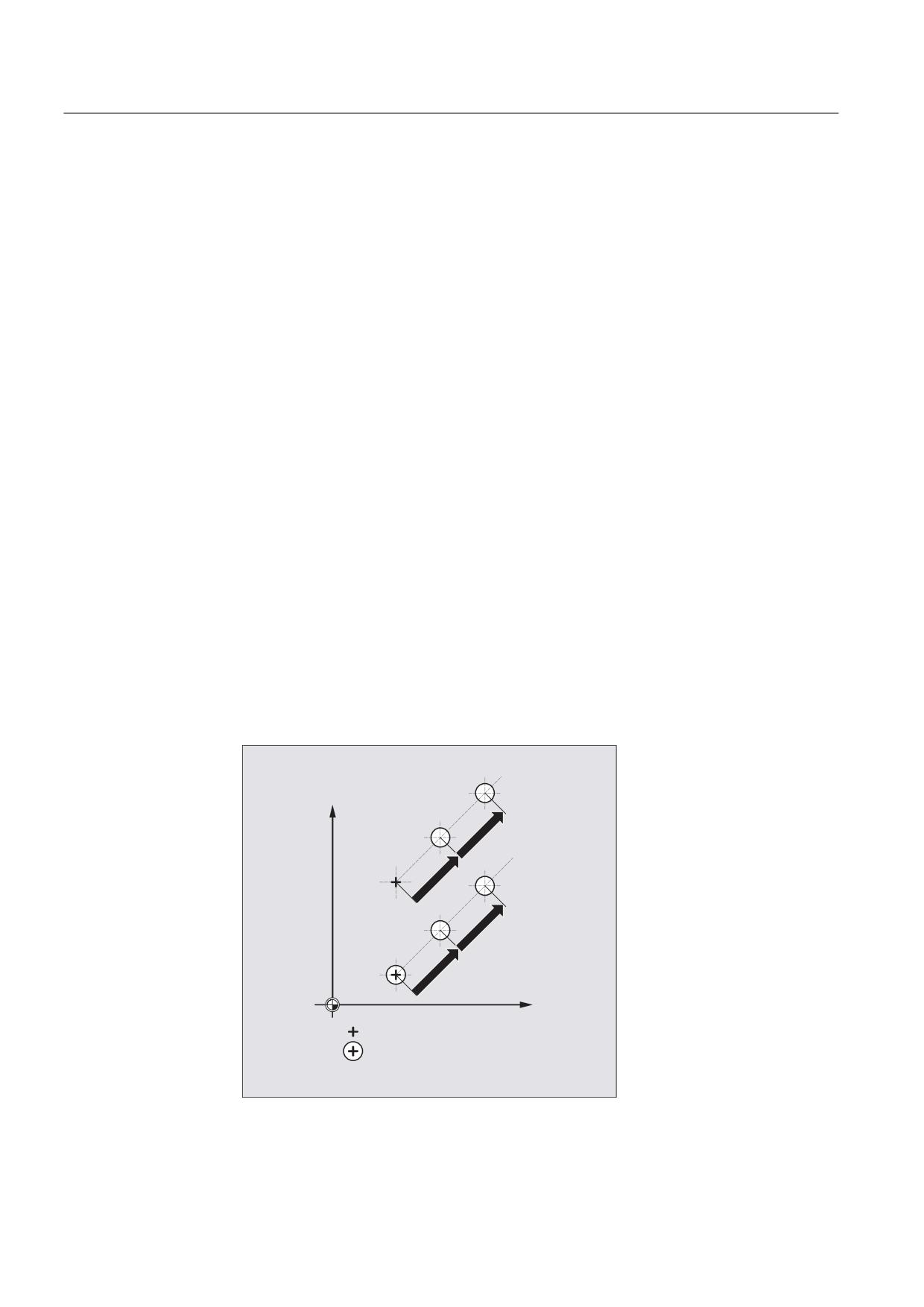
Travel-dependent acceleration (PUNCHACC)
Example:
PUNCHACC(2,50,10,100)
Distance between holes less than 2 mm:
The axis accelerates at a rate corresponding to 50% of maximum acceleration.
Distance between holes from 2 mm to 10 mm:
Acceleration is increased to 100%, proportional to the spacing.
Distance between holes more than 10 mm:
Traverse at an acceleration of 100%.
Initiation of the first stroke
The instant at which the first stroke is initiated after activation of the function differs
depending on whether nibbling or punching is selected:
● PON/PONS:
- All strokes - even the one in the first block after activation - are executed at the block
end.
● SON/SONS:
- The first stroke after activation of the nibbling function is executed at the start of the
block.
- Each of the following strokes is initiated at the block end.
<
321
621
;
3RVLWLRQ
3RVLWLRQLQJ DQG VWURNH UHOHDVH
Job Planning
658
Programming Manual, 03/2010, 6FC5398-2BP20-1BA0
Punching and nibbling
12.1 Activation, deactivation
Punching and nibbling on the spot
A stroke is initiated only if the block contains traversing information for the punching or
nibbling axes (axes in active plane).
However, to initiate a stroke at the same position, one of the punching/nibbling axes can be
programmed with a traversing path of 0.
Machining with rotatable tools
Note
Use the tangential control function if you wish to position rotatable tools at a tangent to the
programmed path.
Use of M commands
As in earlier versions, macro technology allows special M functions to be used instead of
language commands (compatibility). The M functions and equivalent language commands as
used in earlier systems are as follows:
M20, M23
≙ SPOF
M22
≙ SON
M25
≙ PON
M26
≙ PDELAYON
Example for macro file:
Program code
Comment
DEFINE M25 AS PON
; Punching on
DEFINE M125 AS PONS
; Punching with leader on
DEFINE M22 AS SON
; Nibbling on
DEFINE M122 AS SONS
; Nibbling with leader on
DEFINE M26 AS PDELAYON
; Punching with delay on
DEFINE M20 AS SPOF
; Punching/nibbling off
DEFINE M23 AS SPOF
; Punching, nibbling off
Programming example:
Program code
Comment
N100 X100 M20
; Position without punch initiation.
N110 X120 M22
; Activate nibbling, initiate stroke before and
after motion,
N120 X150 Y150 M25
; Activate punching, initiate stroke at end of
motion.
Job Planning
Programming Manual, 03/2010, 6FC5398-2BP20-1BA0
659
Punching and nibbling
12.2 Automatic path segmentation
12.2
Automatic path segmentation
Function
Segmentation into path segments
When punching or nibbling is activated, both SPP as well as also SPN segment the total
traversing section programmed for the path axes into a number of path segments with the
same length (equidistant path segmentation). Internally, each path segment corresponds to
a block.
Number of strokes
When punching, the first stroke is realized at the end point of the first path segment; on the
other hand for nibbling, at the starting point of the first path segment. Therefore the following
numbers are obtained over the complete traversing section:
Punching: Number of strokes = number of path segments
Nibbling: Number of strokes = number of path segments +1
Auxiliary functions
Auxiliary functions are executed in the first of the generated blocks.
Syntax
SPP=
SPN=
Significance
SPP
Size of path segment (maximum distance between strokes); modal
SPN
Number of path segments per block; modally effective
Job Planning
660
Programming Manual, 03/2010, 6FC5398-2BP20-1BA0
Punching and nibbling
12.2 Automatic path segmentation
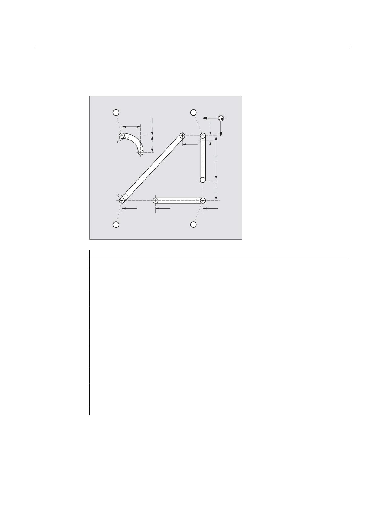
Example 1
The programmed nibbling segments should be automatically split-up into path segments.
;
<
Program code
Comments
N100 G90 X130 Y75 F60 SPOF
; Positioning at starting point 1
N110 G91 Y125 SPP=4 SON
; Nibbling on; maximum path segment
length for automatic path
segmentation: 4 mm (3.81 lb)
N120 G90 Y250 SPOF
; Nibbling off; positioning to
starting point 2
N130 X365 SON
; Nibbling on; maximum path segment
length for automatic path
segmentation: 4 mm (3.81 lb)
N140 X525 SPOF
; Nibbling off; positioning to
starting point 3
N150 X210 Y75 SPP=3 SON
; Nibbling on; maximum path segment
length for automatic path
segmentation: 3 mm (3.81 lb)
N140 X525 SPOF
; Nibbling off; positioning to
starting point 4
N170 G02 X-62.5 Y62.5 I J62.5 SPP=3 SON
; Nibbling on; maximum path segment
length for automatic path
segmentation: 3 mm (3.81 lb)
N180 G00 G90 Y300 SPOF
; Nibbling off
Job Planning
Programming Manual, 03/2010, 6FC5398-2BP20-1BA0
661
Punching and nibbling
12.2 Automatic path segmentation
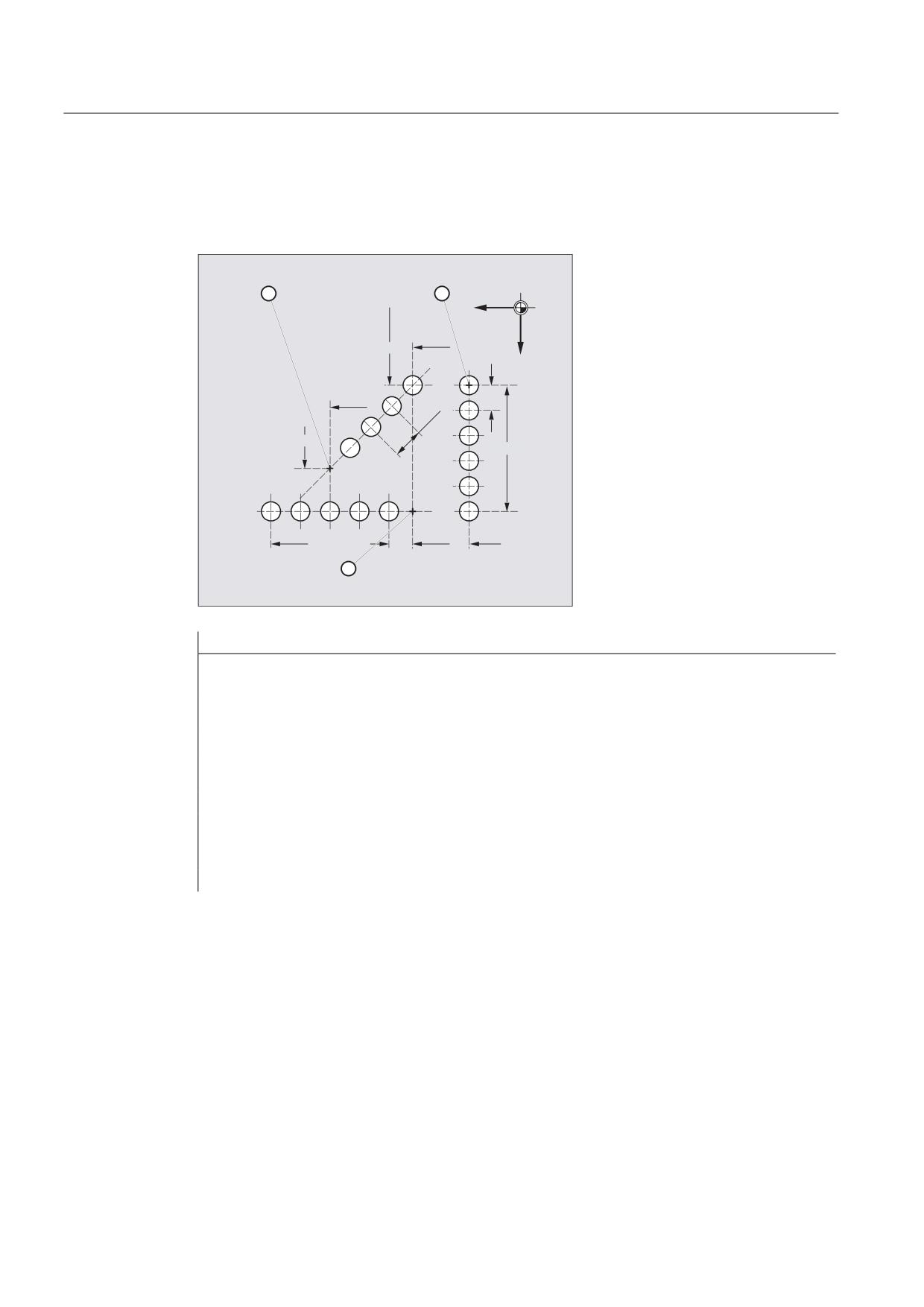
Example 2
Automatic path segmentation should be made for the individual series of holes. The
maximum path segment length (SPP value) is specified for the segmentation.
;
<
Program code
Comments
N100 G90 X75 Y75 F60 PON
;
Position to starting point 1;
punch an individual hole
N110 G91 Y125 SPP=25
;
Maximum path segment length
for automatic path segmentation: 25 mm (3.81 lb)
N120 G90 X150 SPOF
;
Punching off; positioning to starting point 2
N130 X375 SPP=45 PON
;
Punching on; maximum path segment length
for automatic path segmentation: 45 mm (3.81 lb)
N140 X275 Y160 SPOF
;
Punching off; positioning to starting point 3
N150 X150 Y75 SPP=40 PON
;
Punching on, instead of the programmed path segment
length of 40 mm, the ;calculated path segment
length of 37.79 mm is used.
N160 G00 Y300 SPOF
;
Punching off; positioning
Job Planning
662
Programming Manual, 03/2010, 6FC5398-2BP20-1BA0
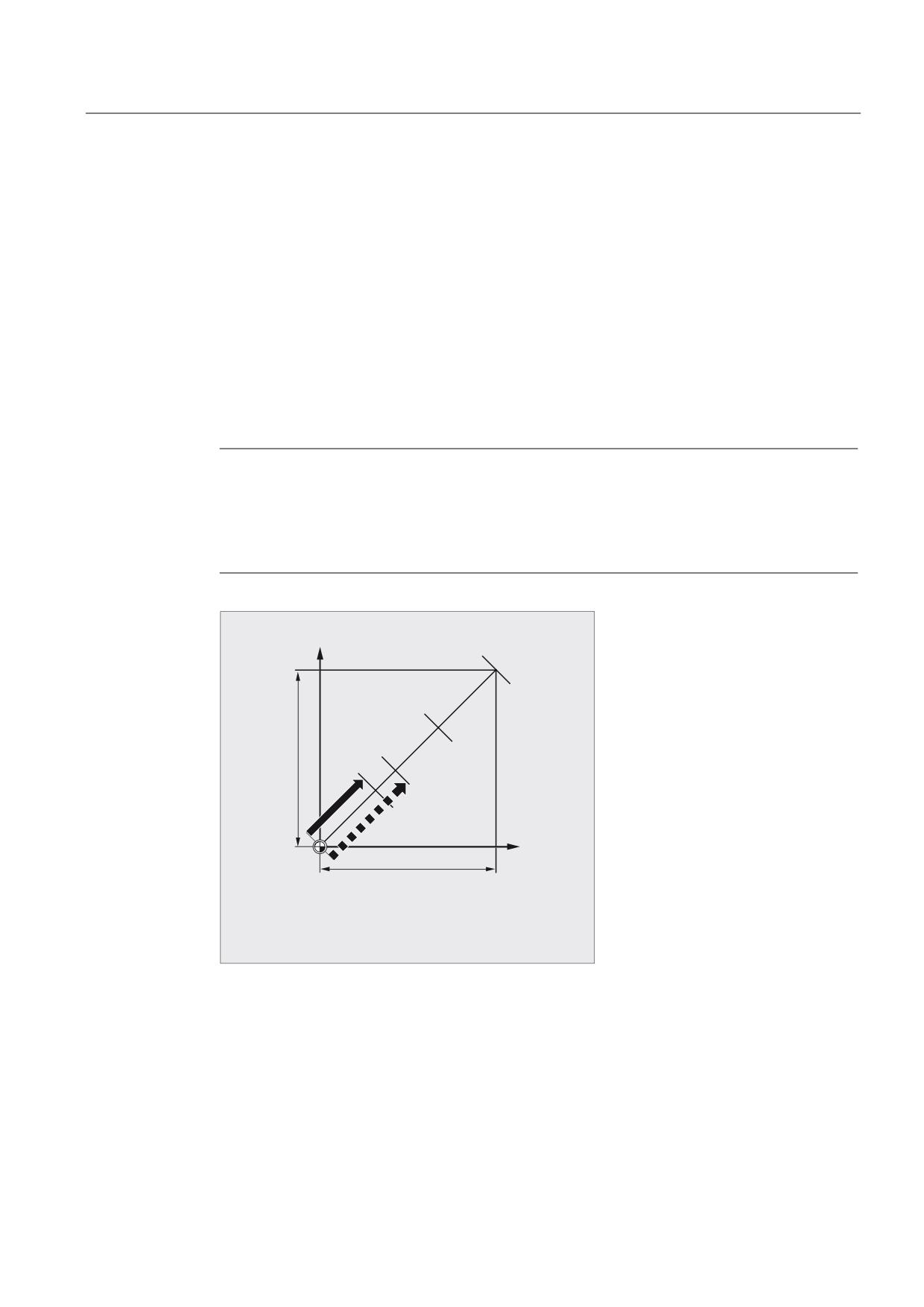
Punching and nibbling
12.2 Automatic path segmentation
12.2.1
Path segmentation for path axes
Length of SPP path segment
SPP is used to specify the maximum distance between strokes and thus the maximum length
of the path segments in which the total traversing distance is to be divided. The command is
deactivated with SPOF or SPP=0.
Example:
N10 SON X0 Y0
N20 SPP=2 X10
The total traversing distance of 10 mm will be divided into five path sections each of 2 mm
(SPP=2).
Note
The path segments effected by SPP are always equidistant, i.e. all segments are equal in
length. In other words, the programmed path segment size (SPP setting) is valid only if the
quotient of the total traversing distance and the SPP value is an integer. If this is not the
case, the size of the path segment is reduced internally such as to produce an integer
quotient.
<
<
(
(
;
;
;
< 3URJUDPPHG WUDYHUVH SDWK QLEEOLQJ RU SXQFKLQJ EORFN
(
3URJUDPPHG SDWK VHJPHQW OHQJWK
(
$XWRPDWLFDOO\ URXQGHG SDWK VHJPHQW OHQJWK
Example:
N10 G1 G91 SON X10 Y10
N20 SPP=3.5 X15 Y15
When the total traversing distance is 15 mm and the path segment length 3.5 mm, the
quotient is not an integer value (4.28). In this case, the SPP value is reduced down to the
next possible integer quotient. The result in this example would be a path segment length of
3 mm.
Job Planning
Programming Manual, 03/2010, 6FC5398-2BP20-1BA0
663
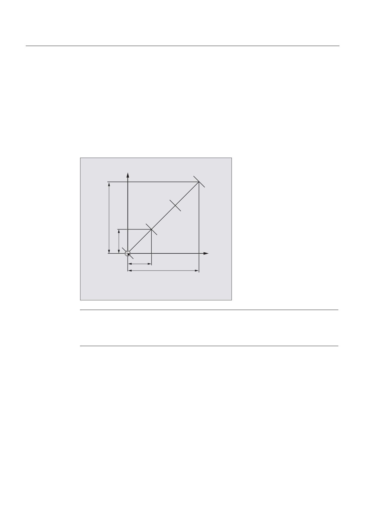
Punching and nibbling
12.2 Automatic path segmentation
Number of SPN path segments
SPN defines the number of path segments to be generated from the total traversing distance.
The length of the segments is calculated automatically. Since SPN is non-modal, punching or
nibbling must be activated beforehand with PON or SON respectively.
SPP and SPN in the same block
If you program both the path segment length (SPP) and the number of path segments (SPN) in
the same block, then SPN applies to this block and SPP to all the following blocks. If SPP was
activated before SPN, then it takes effect again after the block with SPN.
<
<
<
;
;
;
;
<
3URJUDPPHG GLVSODFHPHQW
;
$XWRPDWLFDOO\ FDOFXODWHG SDWK VHFWLRQ LQ
;
<
$XWRPDWLFDOO\ FDOFXODWHG SDWK VHFWLRQ LQ
<
Note
Provided that punching/nibbling functions are available in the control, then it is possible to
program the automatic path segmentation function with SPN or SPP even independent of this
technology.
Job Planning
664
Programming Manual, 03/2010, 6FC5398-2BP20-1BA0
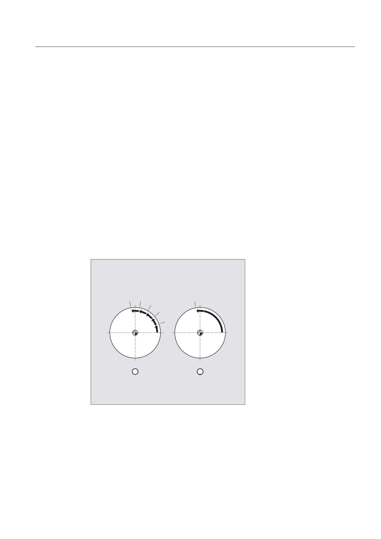
Punching and nibbling
12.2 Automatic path segmentation
12.2.2
Path segmentation for single axes
If single axes are defined as punching/nibbling axes in addition to path axes, then the
automatic path segmentation function can be activated for them.
Response of single axis to SPP
The programmed path segment length (SPP) basically refers to the path axes. For this
reason, the SPP value is ignored in blocks which contain a single axis motion and an SPP
value, but not a programmed path axis.
If both a single axis and a path axis are programmed in the block, then the single axis
responds according to the setting of the appropriate machine data.
1. Standard setting
The path traversed by the single axis is distributed evenly among the intermediate blocks
generated by SPP.
Example:
N10 G1 SON X10 A0
N20 SPP=3 X25 A100
As a result of the programmed distance between strokes of 3 mm, five blocks are generated
for the total traversing distance of the X axis (path axis) of 15 mm.
The A axis thus rotates through 20° in every block.
1. Single axis without path segmentation
The single axis traverses the total distance in the first of the generated blocks.
2. With/without path segmentation
The response of the single axis depends on the interpolation of the path axes:
● Circular interpolation: Path segmentation
● Linear interpolation: No path segmentation
Job Planning
Programming Manual, 03/2010, 6FC5398-2BP20-1BA0
665
Punching and nibbling
12.2 Automatic path segmentation
Response to SPN
The programmed number of path segments is applicable even if a path axis is not
programmed in the same block.
Requirement: The single axis is defined as a punching/nibbling axis.
Job Planning
666
Programming Manual, 03/2010, 6FC5398-2BP20-1BA0
Grinding
13
13.1
Grinding-specific tool monitoring in the part program (TMON, TMOF)
Function
With the TMON command, you can activate geometry and speed monitoring for grinding tools
(type 400 - 499) in the NC part program. Monitoring remains active until deactivated in the
part program using the TMOF command.
Note
Please follow the machine manufacturer's instructions!
Requirements
The grinding-specific tool parameters $TC_TPG1 to $TC_TPG9 must be set.
Syntax
TMON(<T-No.>)
TMOF(<T-No.>)
Description
TMON
Command to switch-in the grinding-specific tool monitoring
TMOF
Command to switch-out the grinding-specific tool monitoring
<T-No.>
Specifies the T number
Note:
Only necessary if the tool with this T number is not active.
TMOF(0)
Deactivate monitoring for all tools
Job Planning
Programming Manual, 03/2010, 6FC5398-2BP20-1BA0
667

Grinding
13.1 Grinding-specific tool monitoring in the part program (TMON, TMOF)
Further Information
Grinding-specific tool parameters
Parameters
Significance
Data type
$TC_TPG1
Spindle number
INT
$TC_TPG2
Chaining rule
INT
The parameters are automatically kept identical for the
lefthand and righthand grinding wheel side.
$TC_TPG3
Minimum wheel radius
REAL
$TC_TPG4
Minimum wheel width
REAL
$TC_TPG5
Current wheel width
REAL
$TC_TPG6
Maximum speed
REAL
$TC_TPG7
Maximum peripheral speed
REAL
$TC_TPG8
Angle of the inclined wheel
REAL
$TC_TPG9
Parameter number for radius calculation
INT
References:
Function Manual Basic Functions; Tool Offset (W1)
Switch-in tool monitoring by selecting a tool
According to the machine data settings, tool monitoring for the grinding tools (types 400-499)
can be automatically activated when the tool selection is activated.
Only one monitoring routine can be active at any one time for each spindle.
Geometry monitoring
The current wheel radius and the current width are monitored.
The set speed is monitored against the speed limitation cyclically with allowance for the
spindle override.
The speed limit is the smaller value resulting from a comparison of the maximum speed with
the speed calculated from the maximum wheel peripheral speed and the current wheel
radius.
Working without a T or D number
A standard T number and standard D number can be set per machine data,
which do not have to be reprogrammed and are effective after power on/reset.
Example: All machining is performed with the same grinding wheel.
The machine data can be used to set that the active tool remains for a reset (see "Free D
number assignment, cutting edge number (Page 429)").
Job Planning
668
Programming Manual, 03/2010, 6FC5398-2BP20-1BA0
Additional functions
14
14.1
Axis functions (AXNAME, AX, SPI, AXTOSPI, ISAXIS, AXSTRING,
MODAXVAL)
Function
AXNAME is used e.g. to generate cycles that are generally valid, if the names of the axes are
not known.
AX is used to indirectly program geometry and synchronous axes. The axis identifier is saved
in a type AXIS variable or is supplied from a command such as AXNAME or SPI.
SPI is used if axis functions are programmed for a spindle, e.g. a synchronous spindle.
AXTOSPI is used to convert an axis identifier into a spindle index (inverse function to SPI).
AXSTRING is used to convert an axis identifier (data type AXIS) into a string (inverse function
to AXNAME).
ISAXIS is used in universal cycles in order to ensure that a specific geometry axis exists and
thus that any following $P_AXNX call is not aborted with an error message.
This MODAXVAL is used in order to determine the modulo position for modulo rotary axes.
Syntax
AXNAME("string")
AX[AXNAME("string")]
SPI(n)
AXTOSPI(A) or AXTOSPI(B) or AXTOSPI(C)
AXSTRING( SPI(n) )
ISAXIS(<geometry axis number>)
<Modulo position>=MODAXVAL(<axis>,<axis position>)
Job Planning
Programming Manual, 03/2010, 6FC5398-2BP20-1BA0
669
Additional functions
14.1 Axis functions (AXNAME, AX, SPI, AXTOSPI, ISAXIS, AXSTRING, MODAXVAL)
Significance
AXNAME
Converts an input string into axis identifiers; the input string must
contain a valid axis name.
AX
Variable axis identifier
SPI
Converts the spindle number into an axis identifier; the transfer
parameter must contain a valid spindle number.
n
Spindle number
AXTOSPI
Converts an axis identifier into an integer spindle index. AXTOSPI
corresponds to the reverse function to SPI.
X, Y, Z
Axis identifier of AXIS type as variable or constant
AXSTRING
The string is output with the associated spindle number.
ISAXIS
Checks whether the specified geometry axis exists.
MODAXVAL
For modulo rotary axes, determines the modulo position; this
corresponds to the modulo rest referred to the parameterized modulo
range (in the default setting, this is 0 to 360 degrees; the start and size
of the modulo range can be changed using MD30340
MODULO_RANGE_START and MD30330 $MA_MODULO_RANGE).
Note
SPI extensions
The axis function SPI(n) can also be used to read and write frame components. This means
that frames can be written e.g. with the syntax $P_PFRAME[SPI(1),TR]=2.22.
An axis can be traversed by additionally programming axis positions using the address
AX[SPI(1)]=<axis position>. The prerequisite is that the spindle is either in the positioning or
axis mode.
Examples
Example 1: AXNAME, AX, ISAXIS
Program code
Comments
OVRA[AXNAME("Transverse axis")]=10
; Override for transverse axis
AX[AXNAME("Transverse axis")]=50.2
; End position for transverse axis
OVRA[SPI(1)]=70
; Override for spindle 1
AX[SPI(1)]=180
; End position for spindle 1
IF ISAXIS(1) == FALSE GOTOF CONTINUE
; Abscissa available?
AX[$P_AXN1]=100
; Move abscissa
CONTINUE:
Job Planning
670
Programming Manual, 03/2010, 6FC5398-2BP20-1BA0
Additional functions
14.1 Axis functions (AXNAME, AX, SPI, AXTOSPI, ISAXIS, AXSTRING, MODAXVAL)
Example 2: AXSTRING
When programming with AXSTRING[SPI(n)], the axis index of the axis, which is assigned to
the spindle, is no longer output as spindle number, but instead the string "Sn" is output.
Program code
Comments
AXSTRING[SPI(2)]
; String "S2" is output.
Example 3: MODAXVAL
The modulo position of modulo rotary axis A is to be determined.
Axis position 372.55 is the starting value for the calculation.
The parameterized modulo range is 0 to 360 degrees:
MD30340 MODULO_RANGE_START = 0
MD30330 $MA_MODULO_RANGE = 360
Program code
Comments
R10=MODAXVAL(A,372.55)
; Calculated modulo position R10 = 12.55.
Example 4: MODAXVAL
If the programmed axis identifier does not refer to a modulo rotary axis, then the value to be
converted (<axis position>) is returned unchanged.
Program code
Comments
R11=MODAXVAL(X,372.55)
; X is a linear axis; R11 = 372.55.
Job Planning
Programming Manual, 03/2010, 6FC5398-2BP20-1BA0
671
Additional functions
14.2 Replaceable geometry axes (GEOAX)
14.2
Replaceable geometry axes (GEOAX)
Function
The "Replaceable geometry axes" function allows the geometry axis grouping configured via
machine data to be modified from the part program. Here any geometry axis can be replaced
by a channel axis defined as a synchronous special axis.
Syntax
GEOAX(<n>,<channel axis>,<n>,<channel axis>,<n>,<channel axis>)
GEOAX()
Significance
GEOAX(...)
Command to change over (replace) the geometry axes
Note:
GEOAX()without any parameter calls the basic configuration of the
geometry axes.
<n>
This parameter is used to specify the number of the geometry axis that
should be assigned to the subsequently specified channel axis.
Range of values:
1, 2, or 3
Note:
With <n>=0, the subsequently specified channel axis can be
completely removed - without any replacement - from the geometry
axis group.
<channel axis>
The parameter is used to specify the name of the channel axis that
should be included in the geometry axis group.
Job Planning
672
Programming Manual, 03/2010, 6FC5398-2BP20-1BA0
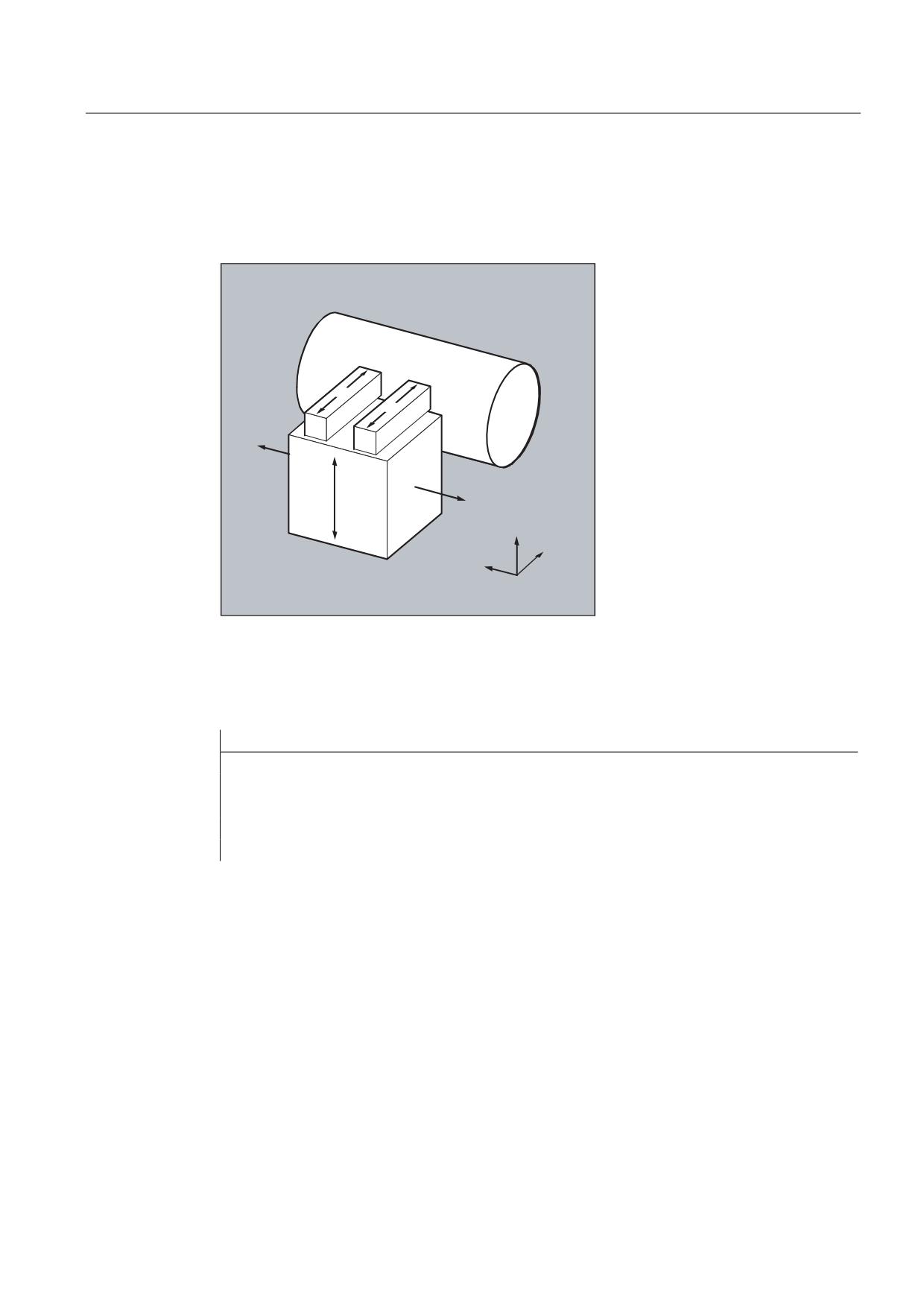
Additional functions
14.2 Replaceable geometry axes (GEOAX)
Examples
Example 1: Switching two axes alternating as geometry axis
A tool slide can be traversed using channel axes X1, Y1, Z1, Z2:
=
=
<
;
<
=
;
The geometry axes are configured so that after powering-up, initially Z1 is effective as 3rd
geometry axis under the geometry axis name "Z" and together with X1 and Y1 forms the
geometry axis group.
Axes Z1 an Z2 should now be used, alternating, as geometry axis Z in the part program:
Program code
Comments
N100 GEOAX(3,Z2)
; Channel axis Z2 acts as 3rd geometry axis (Z).
N110 G1 ...
N120 GEOAX(3,Z1)
; Channel axis Z1 acts as 3rd geometry axis (Z).
Job Planning
Programming Manual, 03/2010, 6FC5398-2BP20-1BA0
673
Additional functions
14.2 Replaceable geometry axes (GEOAX)
Example 2: Changing over the geometry axes for 6 channel axes
A machine has 6 channel axes with the names XX, YY, ZZ, U, V, W.
The basic setting of the geometry axis configuration via machine data is:
Channel axis XX = 1st geometry axis (X axis)
Channel axis YY = 2nd geometry axis (Y axis)
Channel axis ZZ = 3rd geometry axis (Z axis)
Program code
Comments
N10 GEOAX()
; The basic configuration of the geometry axes is
effective.
N20 G0 X0 Y0 Z0 U0 V0 W0
; All axes in rapid traverse to position 0.
N30 GEOAX(1,U,2,V,3,W)
; Channel axis U becomes the first (X), V the second
(Y) and W the third geometry axis (Z).
N40 GEOAX(1,XX,3,ZZ)
; Channel axis XX becomes the first (X), ZZ the third
geometry axis (Z). Channel axis V remains the
second geometry (Y).
N50 G17 G2 X20 I10 F1000
; Full circle in the X/Y plane. Channel axes XX and V
traverse.
N60 GEOAX(2,W)
; Channel axis W becomes the second geometry (Y).
N80 G17 G2 X20 I10 F1000
; Full circle in the X/Y plane. Channel axes XX and W
traverse.
N90 GEOAX()
; Reset to the initial state.
N100 GEOAX(1,U,2,V,3,W)
; Channel axis U becomes the first (X), V the second
(Y) and W the third geometry axis (Z).
N110 G1 X10 Y10 Z10 XX=25
; Channel axes U, V, W each traverse to position 10.
XX as supplementary axis traverses to position 25.
N120 GEOAX(0,V)
; V is removed from the geometry axis group. U and W
remain the first (X) and third geometry axis (Z).
The second geometry (Y) axis remains unassigned.
N130 GEOAX(1,U,2,V,3,W)
; Channel axis U remains the first (X), V becomes the
second (Y), W remains the third geometry axis (Z).
N140 GEOAX(3,V)
; V becomes the third geometry axis (Z), whereby
overwrite W and this is therefore taken out of the
geometry axis group. The second geometry axis (Y)
is, as before, unassigned.
Job Planning
674
Programming Manual, 03/2010, 6FC5398-2BP20-1BA0
Additional functions
14.2 Replaceable geometry axes (GEOAX)
Note
Axis configuration
The machine data below are used to assign the geometry axes, special axes, channel axes
and machine axes as well as the names of the individual axis types:
MD20050 $MC_AXCONF_GEOAX_ASIGN_TAB (assignment of geometry axis to
channel axis)
MD20060 $MC_AXCONF_GEOAX_NAME_TAB (name of the geometry axis in the channel)
MD20070 $MC_AXCONF_MACHAX_USED (machine axis number valid in channel)
MD20080 $MC_AXCONF_CHANAX_NAME_TAB (name of the channel axis in the channel)
MD10000 $MN_AXCONF_MACHAX_NAME_TAB (machine axis name)
MD35000 $MA_SPIND_ASSIGN_TO_MACHAX (assignment of spindle to machine axis)
References:
Function Manual Basic Functions; Axes, Coordinate Systems, Frames (K2)
Restrictions
● It is not possible to switch the geometry axes over during:
- Active transformation
- Active spline interpolation
- Active tool radius compensation
- Active fine tool compensation
● If the geometry axis and the channel axis have the same name, it is not possible to
change the particular geometry axis.
● None of the axes involved in the changeover may be involved in an action that can go
beyond the block limits - e.g.type A positioning axes or for following axes.
● Geometry axes can only be replaced using the command GEOAX if they were already
available when the system was powered-up (this means that no new ones can be
defined).
● An alarm is output if an attempt is made to replace an axis with GEOAX while executing the
contour table (CONTPRON, CONTDCON).
Job Planning
Programming Manual, 03/2010, 6FC5398-2BP20-1BA0
675
Additional functions
14.2 Replaceable geometry axes (GEOAX)
Supplementary conditions
Axis state after replacing
An axis replaced by the changeover in the geometry axis group can be programmed as
supplementary axis after the changeover operation via its channel axis names.
Frames, protection zones, working area limits
All frames, protection zones and working area limits are deleted after changing over the
geometry axes.
Polar coordinates
Replacing the geometry axes with GEOAX sets analog to a level change with G17-G19, the
modal polar coordinates to a value of 0.
DRF, ZO
A possible handwheel offset (DRF) or an external zero offset (ZO) remains effective after the
changeover.
Basic configuration of the geometry axes
The GEOAX() command calls the basic configuration of the geometry axis group.
The system automatically changes back to the basic configuration after POWER ON and
when changing over into the "reference point approach" mode.
Tool length compensation
An active tool length compensation is also effective after the changeover operation.
However, for geometry axes that have been newly added or those where the position has
been replaced, it is still considered not to have been moved through. For the first motion
command for these geometry axes, the resulting traversing distance correspondingly
comprises the sum of the tool length compensation and the programmed traversing distance.
Geometry axes, which retain their position in the axis group after a replacement operation,
also retain their status with respect to tool length compensation.
Geometry axis configuration for active transformation
The geometry axis configuration applicable in an active transformation (defined using
machine data) cannot be changed using the function "replaceable geometry axes".
Should it be necessary to modify the geometry axis configuration in conjunction with
transformations, then this is only possible using an additional transformation.
A geometry axis configuration changed using GEOAX is deleted by activating a transformation.
If the machine data settings for the transformation do not match those for changing over
geometry axes, then the settings in the transformation have priority.
Example:
One transformation active. According to the machine data, the transformation should be kept
for a reset; however, at the same time, for a reset, the basic configuration of geometry axes
should be established. In this particular case, the geometry axis configuration that was
defined with the transformation is kept.
Job Planning
676
Programming Manual, 03/2010, 6FC5398-2BP20-1BA0
Additional functions
14.3 Axis container (AXCTSWE, AXCTSWED)
14.3
Axis container (AXCTSWE, AXCTSWED)
Function
On rotary indexing machines/multi-spindle machines, the axes holding the workpiece move
from one machining unit to the next. Since the machining units are subject to different NCU
channels, the axes holding the workpiece must be dynamically reassigned to the
corresponding NCU channel if there is a change in station/position. Axis containers are used
for this purpose.
Only one workpiece clamping axis/spindle is active on the local machining unit at a time. The
axis container combines the possible connections to all clamping axes/spindles, of which
only one is active at a time for the machining unit.
The available axes that are defined in the axis container can be changed by switching the
entries in the axis container ("axis container rotation") through an increment that can be
entered via setting data (number of slots).
The command AXCTSWE or AXCTSWED is used to call the axis container rotation from the part
program.
Syntax
AXCTSWE(<axis container>)
AXCTSWED(<axis container>)
Significance
AXCTSWE
Command to rotate an axis container
If all of the enable signals of all channels for the axes of the
container are available in the control, the container is rotated with
the container-specific increment saved in the SD41700
$SN_AXCT_SWWIDTH[<container number>].
AXCTSWED
Command to rotate an axis container where just the active
channel is effective (command version for commissioning!)
Note:
The axes entered in the container are only released if the
remaining channels, which have axes in the container, are in the
reset state.
Job Planning
Programming Manual, 03/2010, 6FC5398-2BP20-1BA0
677
Additional functions
14.3 Axis container (AXCTSWE, AXCTSWED)
<axis container>
Identifier of the axis container that should be moved.
Possible data include:
CT<container number> The number of the axis container is
attached to the CT letter combination.
Example: CT3
<container name>
Individual name of the axis container set
using MD12750 $MN_AXCT_NAME_TAB.
Example: A_CONT3
Further Information
Axis container
Can be assigned via the axis container.
● Local axes and/or
● Link axes
Axis containers with link axes are a NCU-cross device (NCU-global) that is coordinated via
the control. It is also possible to have axis containers that are only used for managing local
axes.
References:
Detailed information on configuring axis containers, see:
Function Manual, Extension Functions; Several Control Panels on Multiple NCUs,
Decentralized Systems (B3)
Enable criteria
AXCTSWE( )
Each channel whose axes are entered in the specified container issues an enable for a
container rotation if it has finished machining the position/station. If the enable signals of
allchannels for the axes of the container have been received in the control, the container is
rotated with the container-specific increment saved in the SD41700
$SN_AXCT_SWWIDTH[<container number>].
Job Planning
678
Programming Manual, 03/2010, 6FC5398-2BP20-1BA0
Additional functions
14.3 Axis container (AXCTSWE, AXCTSWED)
Example:
&KDQQHO D[LV
1R LQ WKH ORJLFDO
/RJLFDO
QDPH
PDFKLQH D[LV LPDJH
PDFKLQH D[LV LPDJH
;
$;
> @ /RFDO PDFKLQH D[LV
<
$;
> @ /RFDO PDFKLQH D[LV
=
6
&7 B6/
> @ $[LV FRQWDLQHU HQWU\
6ORW
$[LV FRQWDLQHU
$[LV FRQWDLQHU
1& B$;
1& B$;
1& B$;
1& B$;
1& B$;
1& B$;
$;&76:( &7
1& B$;
1& B$;
$[LV FRQWDLQHU HQWULHV VKLIWHG
E\ DQ LQFUHPHQW RI
After the axis container is rotated through 1, channel axis Z is assigned to axis AX5 on NCU
1 instead of axis AX1 on NCU.
AXCTSWED( )
The command version AXCTSWED() can be used to simplify commissioning. The axis container
rotates with just the active channel being effective through the container-specific increment
saved in SD41700 $SN_AXCT_SWWIDTH[<container number>]. This call may only be used
if the remaining channels, that have axes in the container, are in the reset state.
Effectiveness
After an axis container rotation, all NCUs are involved in the new axis assignment whose
channels refer to the rotated axis container via the logical machine axis image.
Job Planning
Programming Manual, 03/2010, 6FC5398-2BP20-1BA0
679
Additional functions
14.3 Axis container (AXCTSWE, AXCTSWED)
Axis container revolution with implicit GET/GETD
When an axis container revolution is enabled, all axis container axes assigned to the
channel are assigned to the channel with GET or GETD. Axes cannot be released until the axis
container has been rotated.
Note
This behavior can be set using machine data. Please refer to the machine manufacturer's
instructions.
Note
Axis container rotation with implicit GET / GETD cannot be used for an axis in the state main
run axis, (e.g. for a PLC axis) as this axis would have to exit the main run status for the
purpose of axis container rotation.
Job Planning
680
Programming Manual, 03/2010, 6FC5398-2BP20-1BA0
Additional functions
14.4 Wait for valid axis position (WAITENC)
14.4
Wait for valid axis position (WAITENC)
Function
Using the language command WAITENC, the NC program waits until the synchronized or
restored axis positions are available for the axes configured with
MD34800 $MA_WAIT_ENC_VALID = 1.
An interruption can take place in the wait state, e.g. by starting an ASUB or by changing the
operating mode to JOG. When the program is continued, where relevant, the wait state is
resumed.
Note
In the user interface, the wait state is displayed using the hold state "Wait for measuring
system".
Syntax
WAITENC can be programmed in the program section of any NC program.
Programming must be realized in a dedicated block:
WAITENC
Example
WAITENC is e.g. used in an event-controlled user program,
.../_N_CMA_DIR/_N_PROG_EVENT_SPF, as shown in the following application example.
Application example:Tool retraction after POWER OFF with orientation transformation
Machining with tool orientation was interrupted due to a power failure.
When powering up again, the event-controlled user program
.../_N_CMA_DIR/_N_PROG_EVENT_SPF is called.
In the event-controlled user program, the system waits for synchronized or restored axis
positions using WAITENC; in order to then be able to calculate a frame, which aligns the WCS
in the tool direction.
Job Planning
Programming Manual, 03/2010, 6FC5398-2BP20-1BA0
681