SINUMERIK 840D sl/828D. Job Planning. Programming Manual (2010-2018)

Path traversing behavior

8.5 Preventing program position for SERUPRO (IPTRLOCK, IPTRUNLOCK)

Rules for nesting

The following features regulate the interaction between NC commands IPTRLOCK and

IPTRUNLOCK with nesting and end of subroutine:

1. IPTRLOCK is activated implicitly at the end of the subroutine in which IPTRUNLOCK is called.

2. IPTRLOCK in an untraceable section has no effect.

3. If subroutine 1 calls subroutine 2 in an untraceable section, the whole of subroutine 2

remains untraceable. IPTRUNLOCK in particular has no effect in subroutine 2.

For more information, see

/FB1/ Function Manual, Basic Functions; Mode Group, Channel, Program Operation Mode (K1).

System variables

An untraceable section can be detected in the parts program with $P_IPTRLOCK.

Automatic interrupt pointer

The automatic interrupt pointer automatically defines a previously defined coupling type as

untraceable. The machine data for

● electronic gearbox with EGON

● axial leading value coupling with LEADON

are used to activate the automatic interrupt pointer. If the programmed interrupt pointer and

interrupt pointer activated with automatic interrupt pointers overlap, the largest possible

untraceable section will be generated.

Job Planning

Programming Manual, 03/2010, 6FC5398-2BP20-1BA0

475

Path traversing behavior

8.6 Repositioning to a contour (REPOSA, REPOSL, REPOSQ, REPOSQA, REPOSH, REPOSHA, DISR,

DISPR, RMI, RMB, RME, RMN)

8.6

Repositioning to a contour (REPOSA, REPOSL, REPOSQ,

REPOSQA, REPOSH, REPOSHA, DISR, DISPR, RMI, RMB, RME,

RMN)

Function

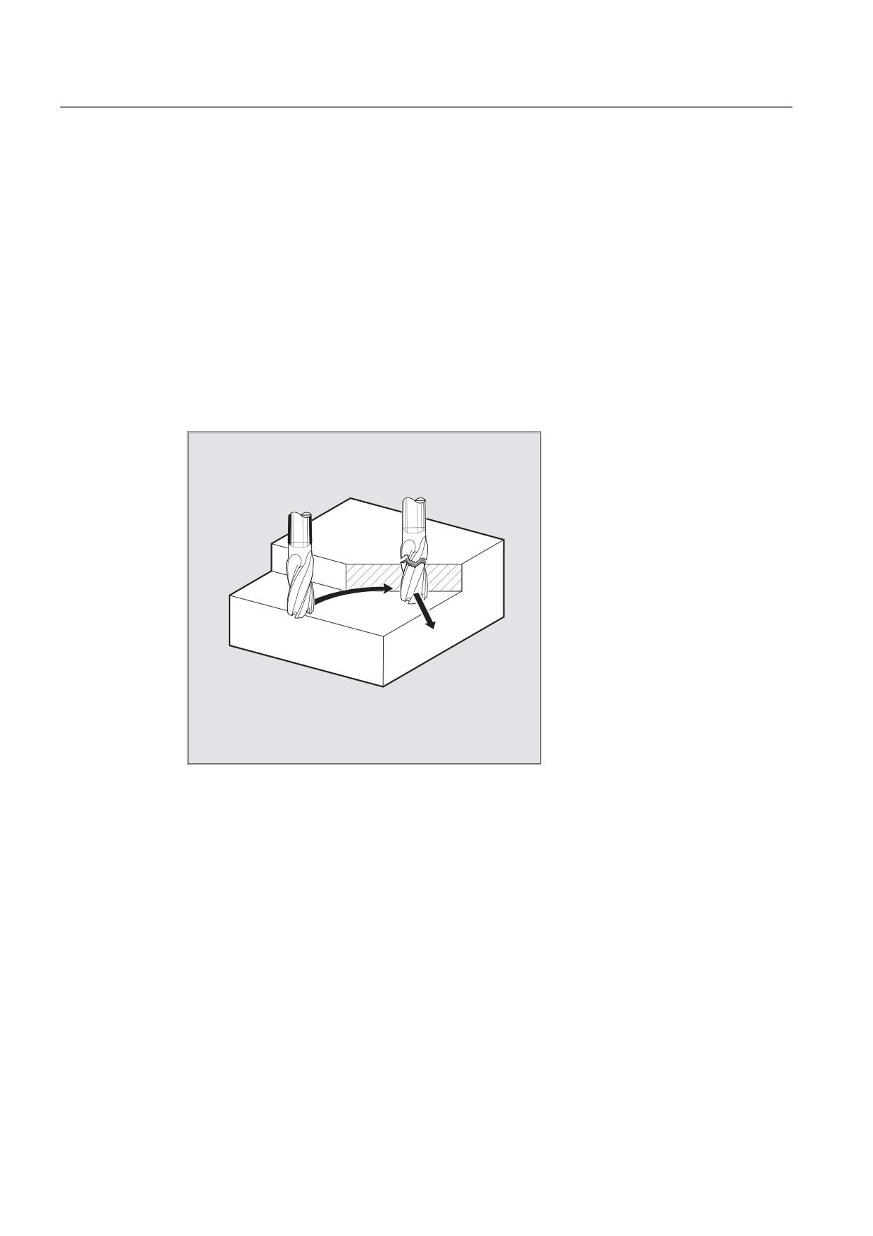
If you interrupt the program run and retract the tool during the machining operation because,

for example, the tool has broken or you wish to check a measurement, you can reposition at

any selected point on the contour under control by the program.

The REPOS command acts in the same way as a subprogram return jump (e.g., via M17).

Blocks programmed after the command in the interrupt routine are not executed.

5(326

For information about interrupting program runs, see also Section "Flexible NC

programming", Chapter "Interrupt routine" in this Programming Manual.

Job Planning

476

Programming Manual, 03/2010, 6FC5398-2BP20-1BA0

Path traversing behavior

8.6 Repositioning to a contour (REPOSA, REPOSL, REPOSQ, REPOSQA, REPOSH, REPOSHA, DISR, DISPR, RMI, RM

Syntax

REPOSA RMI DISPR=…

REPOSA RMB

REPOSA RME

REPOSA RMN

REPOSL RMI DISPR=…

REPOSL RMB

REPOSL RME

REPOSL RMN

REPOSQ RMI DISPR=… DISR=…

REPOSQ RMB DISR=…

REPOSQ RME DISR=…

REPOSQA DISR=…

REPOSH RMI DISPR=… DISR=…

REPOSH RMB DISR=…

REPOSH RME DISR=…

REPOSHA DISR=…

Significance

Approach path

REPOSA

Approach along line on all axes

REPOSL

Approach along line

REPOSQ DISR=…

Approach along quadrant with radius DISR

REPOSQA DISR=…

Approach on all axes along quadrant with radius DISR

REPOSH DISR=…

Approach along semi-circle with diameter DISR

REPOSHA DISR=…

Approach on all axes along semi-circle with diameter DISR

Reapproach point

RMI

Approach interruption point

RMI DISPR=…

Entry point at distance DISPR in mm/inch in front of interruption

point

RMB

Approach block start point

RME

Approach end of block

RME DISPR=…

Approach block end point at distance DISPR in front of end

point

RMN

Approach at nearest path point

A0 B0 C0

Axes in which approach is to be made

Job Planning

Programming Manual, 03/2010, 6FC5398-2BP20-1BA0

477

Path traversing behavior

8.6 Repositioning to a contour (REPOSA, REPOSL, REPOSQ, REPOSQA, REPOSH, REPOSHA, DISR,

DISPR, RMI, RMB, RME, RMN)

Example: Approach along a straight line, REPOSA, REPOSL

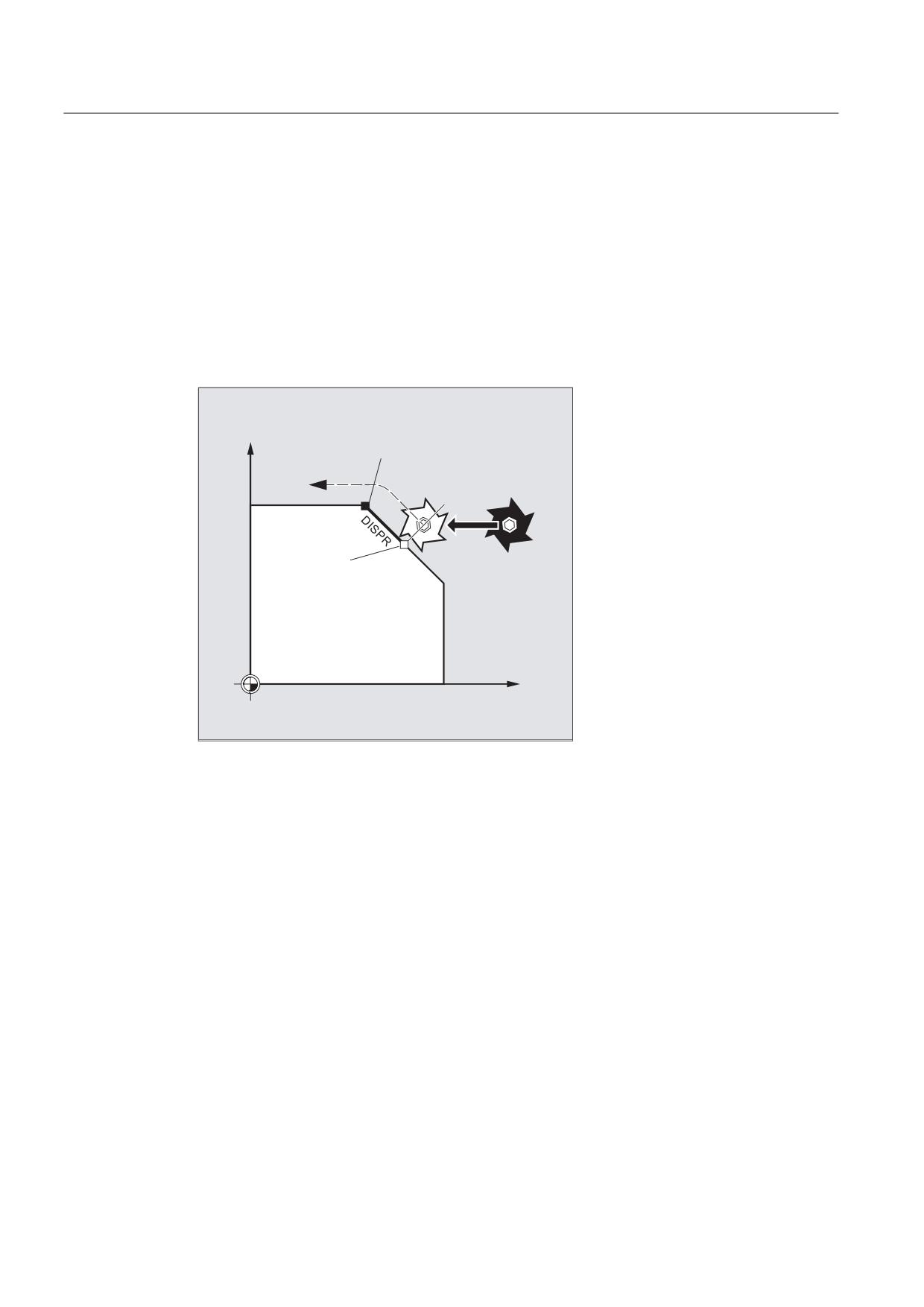
The tool approaches the repositioning point along a straight line.

All axes are automatically traversed with command REPOSA. With REPOSL you can specify

which axes are to be moved.

Example:

REPOSL RMI DISPR=6 F400

REPOSA RMI DISPR=6 F400

,QWHUUXSWLRQ SRLQW

5(326/

%ORFN VWDUW SRLQW

;

Job Planning

478

Programming Manual, 03/2010, 6FC5398-2BP20-1BA0

Path traversing behavior

8.6 Repositioning to a contour (REPOSA, REPOSL, REPOSQ, REPOSQA, REPOSH, REPOSHA, DISR, DISPR, RMI, RM

Example: Approach in circle quadrant, REPOSQ, REPOSQA

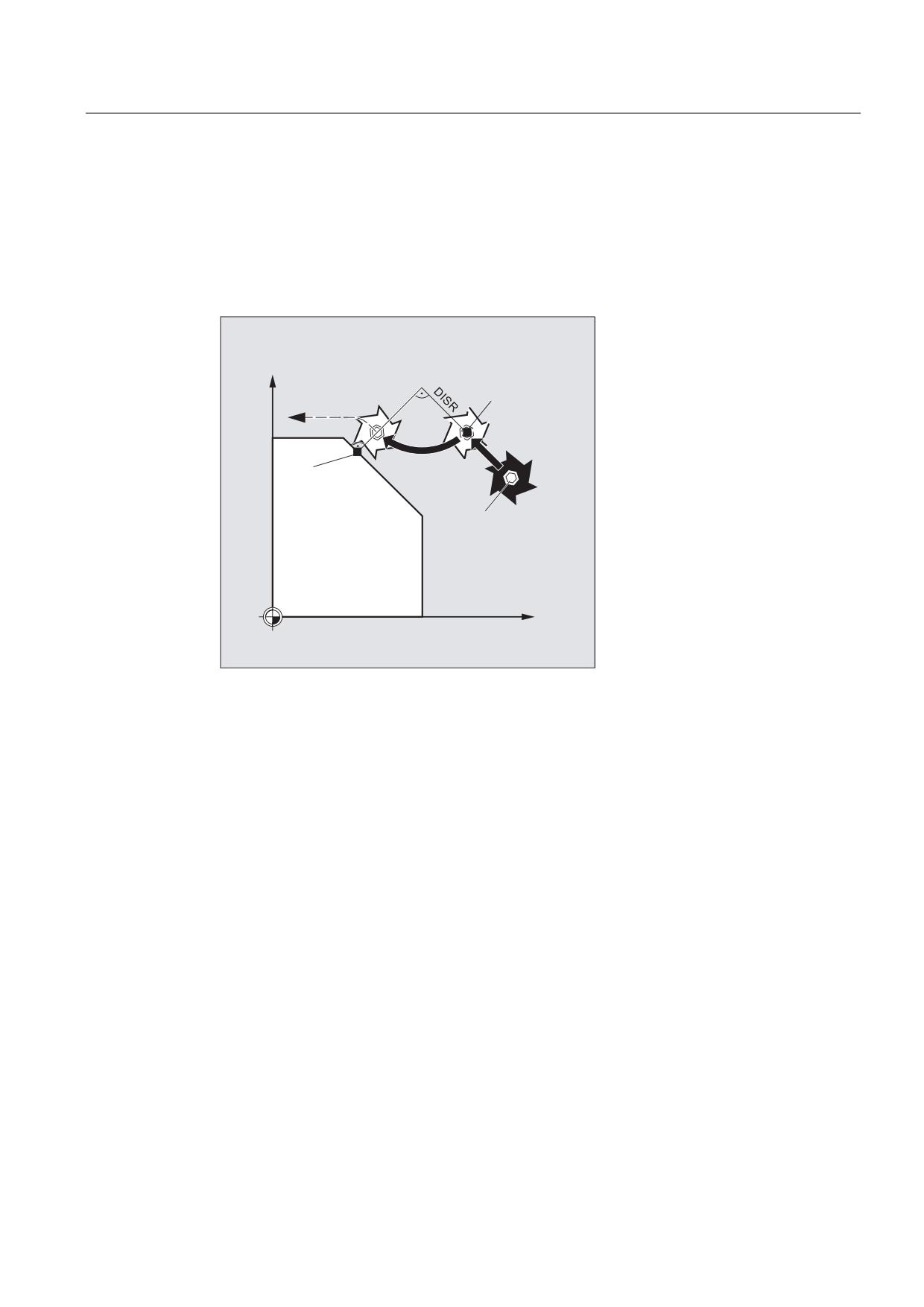
The tool approaches the repositioning point along a quadrant with a radius of DISR=…. The

control system automatically calculates the intermediate point between the start and

repositioning points.

Example:

REPOSQ RMI DISR=10 F400

,QWHUPHGLDWH

SRLQW

(32 6

%ORFN VWDUW SRLQW

6WDUW SRLQW

;

Job Planning

Programming Manual, 03/2010, 6FC5398-2BP20-1BA0

479

Path traversing behavior

8.6 Repositioning to a contour (REPOSA, REPOSL, REPOSQ, REPOSQA, REPOSH, REPOSHA, DISR,

DISPR, RMI, RMB, RME, RMN)

Example: Approach tool in a semicircle, REPOSH, REPOSHA

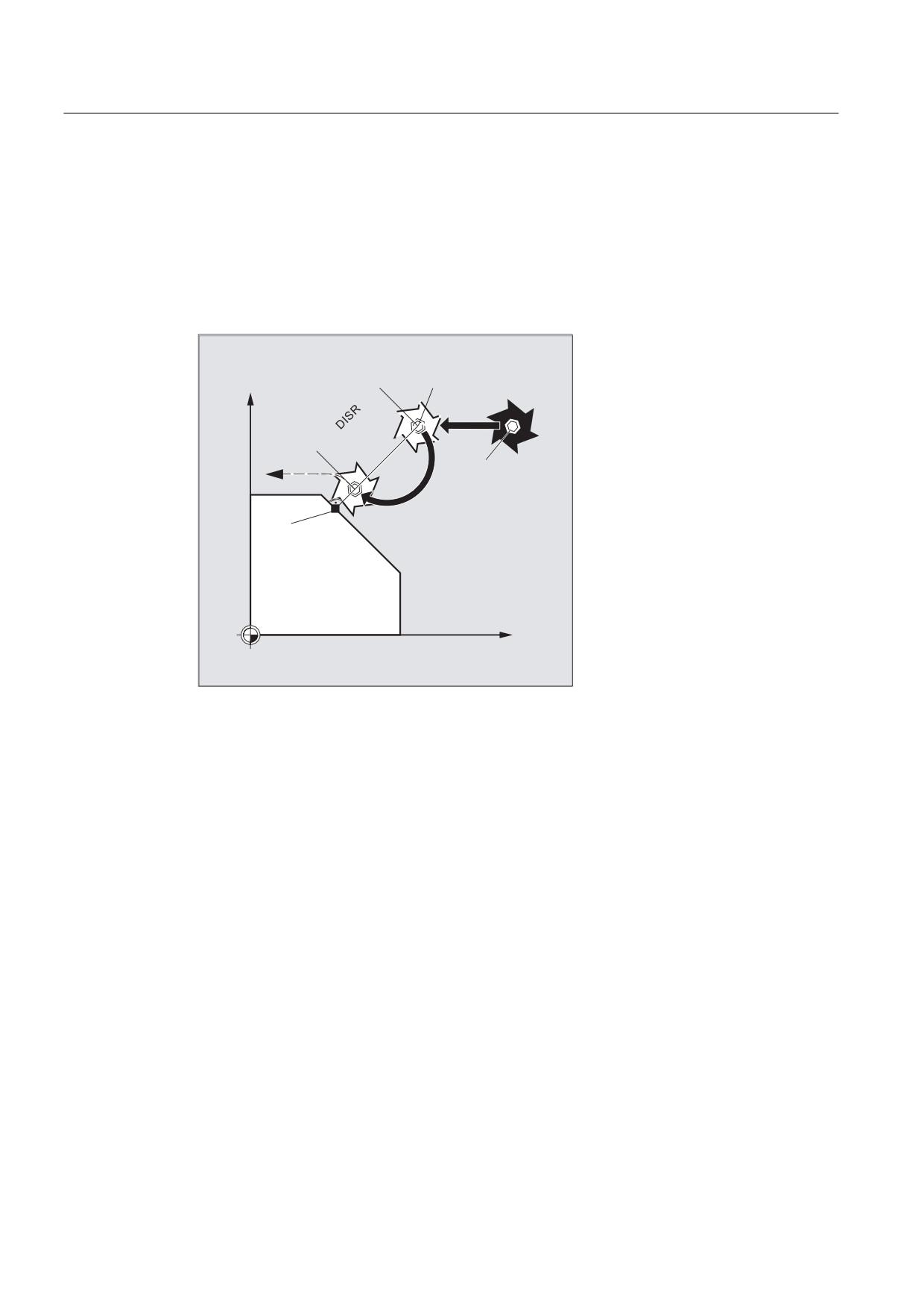
The tool approaches the repositioning point along a semi-circle with a diameter of DISR=….

The control automatically calculates the necessary intermediate point between the start and

repositioning point.

Example:

REPOSH RMI DISR=20 F400

,QWHUPHGLDWH SRLQW

6WDUW SRLQW

%ORFN VWDUW SRLQW

;

Job Planning

480

Programming Manual, 03/2010, 6FC5398-2BP20-1BA0

Path traversing behavior

8.6 Repositioning to a contour (REPOSA, REPOSL, REPOSQ, REPOSQA, REPOSH, REPOSHA, DISR, DISPR, RMI, RM

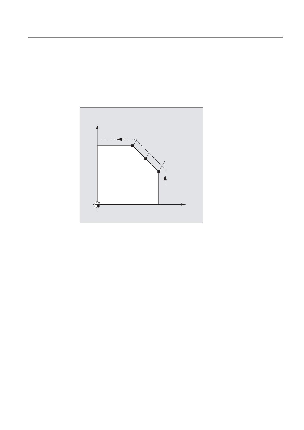
Specifying the repositioning point (not for SERUPRO approaching with RMN)

With reference to the NC block in which the program run has been interrupted, it is possible

to select one of three different repositioning points:

● RMI, interruption point

● RMB, block start point or last end point

● RME, block end point

%ORFN HQG SRLQW

,QWHUUXSWLRQ SRLQW

50(

%ORFN VWDUW SRLQW

50,

50%

;

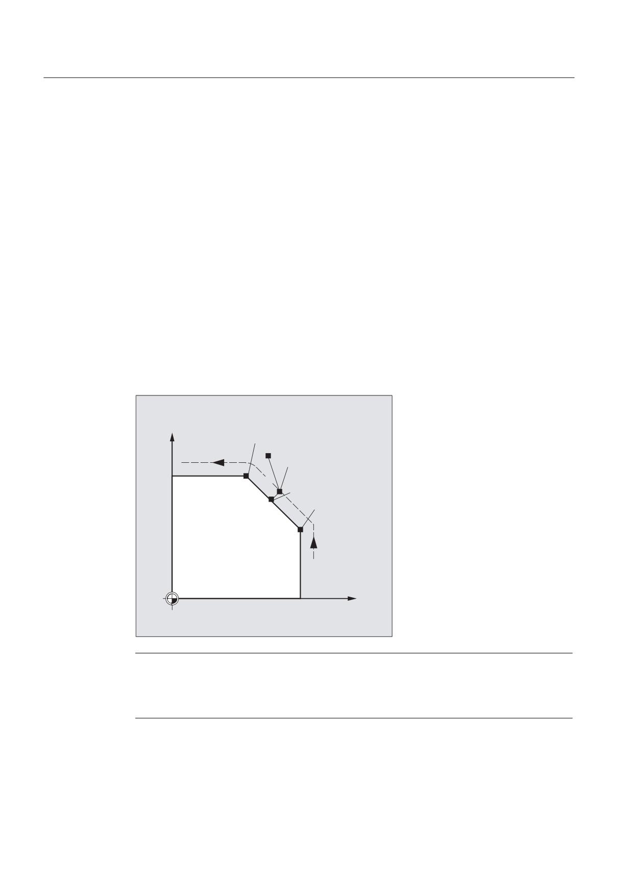
RMI DISPR=… or RME DISPR=… allows you to select a repositioning point which sits before the

interruption point or the block end point.

DISPR=… allows you to describe the contour distance in mm/inch between the repositioning

point and the interruption before the end point. Even for high values, this point cannot be

further away than the block start point.

If no DISPR=… command is programmed, then DISPR=0 applies and with it the interruption point

(with RMI) or the block end point (with RME).

Job Planning

Programming Manual, 03/2010, 6FC5398-2BP20-1BA0

481

Path traversing behavior

8.6 Repositioning to a contour (REPOSA, REPOSL, REPOSQ, REPOSQA, REPOSH, REPOSHA, DISR,

DISPR, RMI, RMB, RME, RMN)

DISPR sign

The sign DISPR is evaluated. In the case of a plus sign, the behavior is as previously.

In the case of a minus sign, approach is behind the interruption point or, with RMB, behind the

block start point.

The distance between interruption point and approach point depends on the value of DISPR.

Even for higher values, this point can lie in the block end point at the maximum.

Sample application:

A sensor will recognize the approach to a clamp. An ASUP is initiated to bypass the clamp.

Afterwards, a negative DISPR is repositioned on one point behind the clamp and the program

is continued.

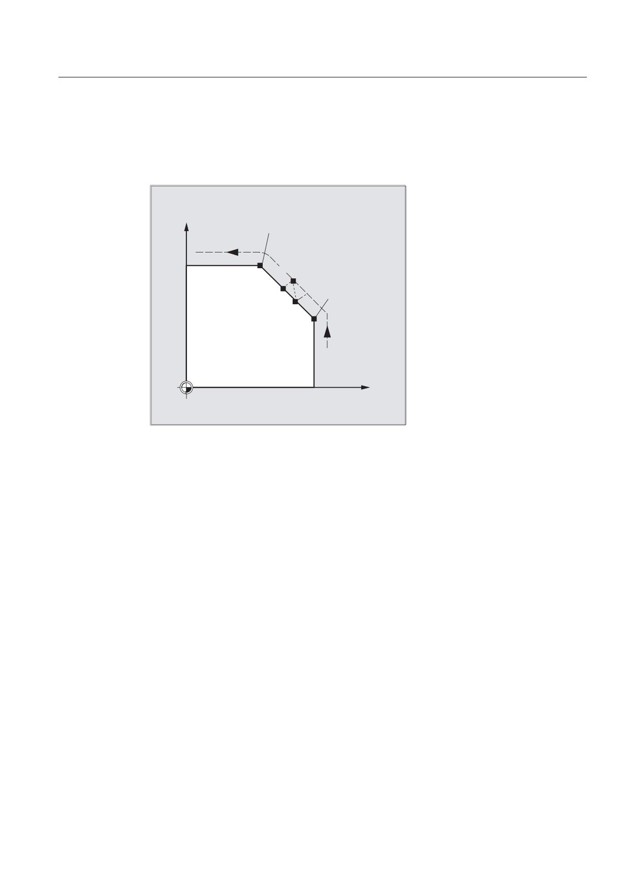
SERUPRO approach with RMN

If abort is forced during machining at any position, the shortest path from the abort point is

approached with SERUPRO approach and RMN so that afterward only the distance-to-go is

processed. The user starts a SERUPRO process at the interruption block and uses the JOG

keys to move in front of the problem component of the target block.

%ORFN HQG SRLQW

$FWXDO SRVLWLRQ IRU EORFN VHDUFK

3RVLWLRQ UHDFKHG XVLQJ

-2* NH\

50(

6(58352 DSSURDFK

501

%ORFN VWDUW SRLQW

50,

50%

;

Note

SERUPRO

For SERUPRO, RMI and RMB are identical. RMN is not limited to SERUPRO but is generally

applicable.

Job Planning

482

Programming Manual, 03/2010, 6FC5398-2BP20-1BA0

Path traversing behavior

8.6 Repositioning to a contour (REPOSA, REPOSL, REPOSQ, REPOSQA, REPOSH, REPOSHA, DISR, DISPR, RMI, RM

Approach from the nearest path point RMN

When REPOSA is interpreted, the repositioning block with RMN is not started again in full after

an interruption, but only the distance-to-go processed. The nearest path point of the

interrupted block is approached.

%ORFN HQG SRLQW

50(

5HSRVLWLRQLQJ

$68%

501

%ORFN VWDUW SRLQW

50,

50%

;

Status for the valid REPOS mode

The valid REPOS mode of the interrupted block can be read with synchronized actions and

variable $AC_ REPOS_PATH_MODE:

0: Approach not defined

1 RMB: Approach to beginning

2 RMI: Approach to point of interruption

3 RME: Approach to end of block

4 RMN: Approaching to next path point of the interrupted block

Job Planning

Programming Manual, 03/2010, 6FC5398-2BP20-1BA0

483

Path traversing behavior

8.6 Repositioning to a contour (REPOSA, REPOSL, REPOSQ, REPOSQA, REPOSH, REPOSHA, DISR,

DISPR, RMI, RMB, RME, RMN)

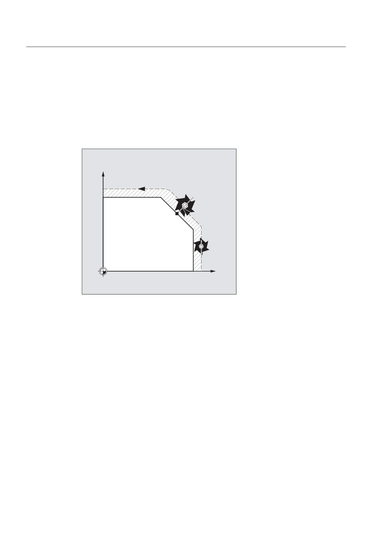
Approaching with a new tool

The following applies if you have stopped the program run due to tool breakage:

When the new D number is programmed, the machining program is continued with modified

tool offset values at the repositioning point.

Where tool offset values have been modified, it may not be possible to reapproach the

interruption point. In such cases, the point closest to the interruption point on the new

contour is approached (possibly modified by DISPR).

;

Approach contour

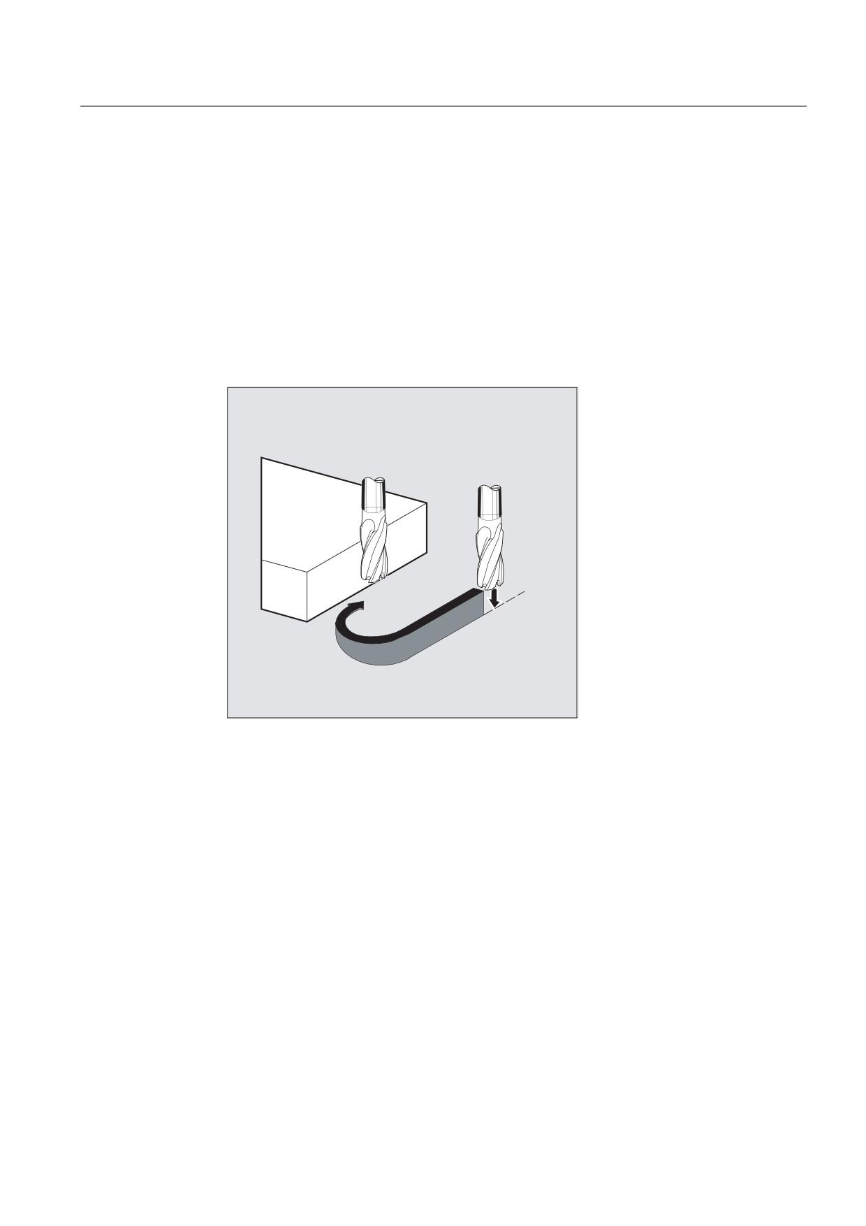
The motion with which the tool is repositioned on the contour can be programmed. Enter

zero for the addresses of the axes to be traversed.

The REPOSA, REPOSQA and REPOSHA commands automatically reposition all axes. Individual

axis names need not be specified.

When the commands REPOSL, REPOSQ and REPOSH are programmed, all geometry axes are

traversed automatically, i.e. they need not be named in the command. All other axes must be

specified in the commands.

Job Planning

484

Programming Manual, 03/2010, 6FC5398-2BP20-1BA0

Path traversing behavior

8.6 Repositioning to a contour (REPOSA, REPOSL, REPOSQ, REPOSQA, REPOSH, REPOSHA, DISR, DISPR, RMI, RM

The following applies to the REPOSH and REPOSQ circular motions:

The circle is traversed in the specified working planes G17 to G19.

If you specify the third geometry axis (infeed direction) in the approach block, the

repositioning point is approached along a helix in case the tool position and programmed

position in the infeed direction do not coincide.

In the following cases, the control automatically switches over to linear approach REPOSL:

● You have not specified a value for DISR.

● No defined approach direction is available (program interruption in a block without travel

information).

● With an approach direction that is perpendicular to the current working plane.

Job Planning

Programming Manual, 03/2010, 6FC5398-2BP20-1BA0

485

Path traversing behavior

8.7 Influencing the motion control

8.7

Influencing the motion control

8.7.1

Percentage jerk correction (JERKLIM)

Function

Using the NC command JERKLIM, the maximum jerk of an axis for path motion - set using

machine data - can be reduced or increased in critical program sections.

Precondition

The acceleration mode SOFT must be active.

Effectiveness

The function is effective:

● In the AUTOMATIC operating modes.

● Only on path axes.

Syntax

JERKLIM[<axis>]=<value>

Meaning

JERKLIM:

Command for jerk correction

<axis>:

Machine axis whose jerk limit value is to be adapted.

<value>

Percentage correction value, referred to the configured maximum axis

jerk for path motion (MD32431 $MA_MAX_AX_JERK).

Range of values:

1 ... 200

Value 100 does not influence the jerk.

Note

The behavior of JERKLIM at the end of the part program and channel reset is configured

with bit 0 in machine data MD32320 $MA_DYN_LIMIT_RESET_MASK:

• Bit 0 = 0:

The programmed value for JERKLIM is reset to 100% with channel reset/M30.

• Bit 0 = 1:

The programmed value for JERKLIM is retained beyond the channel reset/M30.

Job Planning

486

Programming Manual, 03/2010, 6FC5398-2BP20-1BA0

Path traversing behavior

8.7 Influencing the motion control

Example

Program code

Comment

N60 JERKLIM[X]=75

; The axis slide in the X direction should only be

accelerated/decelerated with a maximum of 75% of the

jerk permissible for the axis.

8.7.2

Percentage velocity correction (VELOLIM)

Function

Using the NC command VELOLIM, the maximum possible velocity of an axis/spindle in axis

operation or the maximum possible gear unit-stage dependent speed of a spindle in spindle

operation - set using machine data - (speed control mode M3, M4, M5 and positioning mode

SPOS, SPOSA, M19) can be reduced in critical program sections, e.g. to reduce the stress

on the machine or to improve the machining quality.

Effectiveness

The function is effective:

● in the AUTOMATIC operating modes

● on path and positioning axes

● on spindles in spindle/axis operations

Syntax

VELOLIM[<axis/spindle>]=<value>

Job Planning

Programming Manual, 03/2010, 6FC5398-2BP20-1BA0

487

Path traversing behavior

8.7 Influencing the motion control

Meaning

VELOLIM:

Command for velocity correction

<axis/spindle>:

Machine axis or spindle whose velocity or speed limit value should

be adapted.

VELOLIM for spindles

Using machine data (MD30455 $MA_MISC_FUNCTION_MASK,

bit 6), when programming in the part program, it can be set as to

whether VELOLIM is effective independent of whether used as

spindle or axis (bit 6 = 1) - or is able to be programmed separately

for each operating mode (bit 6 = 0). If they are to be separately

effective, then the selection is made using the identifier when

programming:

• Spindle identifier S<n> for spindle operating modes

• Axis identifier, e.g. "C", for axis operation

<value>:

Percentage correction value

The correction value refers to:

• for axes / spindles in axis operation (if MD30455 bit 6 = 0):

to the configured maximum axis velocity

(MD32000 $MA_MAX_AX_VELO).

• for spindles in spindle or axis operation (if MD30455 bit 6 = 1):

to the maximum speed of the active gear unit stage

(MD35130 $MA_GEAR_STEP_MAX_VELO_LIMIT[<n>])

Range of values:

1 ... 100

The value 100 does not influence the velocity or speed.

Note

Behavior at the end of the part program and for a channel reset

The behavior of VELOLIM at the end of the part program and channel reset is configured

with bit 0 in machine data MD32320 $MA_DYN_LIMIT_RESET_MASK:

• Bit 0 = 0:

The programmed value for VELOLIM is reset to 100% with channel reset/M30.

• Bit 0 = 1:

The programmed value for VELOLIM is retained beyond the channel reset/M30.

Job Planning

488

Programming Manual, 03/2010, 6FC5398-2BP20-1BA0

Path traversing behavior

8.7 Influencing the motion control

Note

VELOLIM for spindles in synchronized actions

When programming VELOLIM in synchronized actions, a distinction is not made between

spindle and axis operation. Independent of the identifiers used when programming, the

speed in spindle operation and the velocity in axis operation are limited to the same extent.

Diagnostics

VELOLIM diagnostics in spindle operation

Active speed limiting using VELOLIM (less than 100 %) can be identified in spindle operation

by reading the system variables $AC_SMAXVELO and $AC_SMAXVELO_INFO.

In the case of limiting, $AC_SMAXVELO supplies the speed limit generated by VELOLIM. In

this case, variable $AC_SMAXVELO_INFO returns the value "16" as identifier for the cause

of the limit VELOLIM.

Examples

Example 1: Velocity limiting, machine axis

Program code

Comment

N70 VELOLIM[X]=80

; The axis slide in the X direction should only be

traversed with a maximum of 80% of the velocity

permissible for the axis.

Example 2: Speed limiting, spindle

Program code

Comment

N05 VELOLIM[S1]=90

; Limiting the maximum speed of spindle 1 to 90% of

1000 rpm.

N50 VELOLIM[C]=45

; Limiting the speed to 45% of 1000 rpm, C is the axis

identifier of S1.

Job Planning

Programming Manual, 03/2010, 6FC5398-2BP20-1BA0

489

Path traversing behavior

8.7 Influencing the motion control

Configuring data for spindle 1 (AX5):

MD35130 $MA_GEAR_STEP_MAX_VELO_LIMIT[1,AX5]=1000

; Maximum speed of

gear unit stage 1 =

1000 rpm

MD30455 $MA_MISC_FUNCTION_MASK[AX5] = 64

; Bit 6 = 1:

Programming VELOLIM

acts together for

spindle and axis

operation

independent of the

programmed

identifier.

8.7.3

Program example for JERKLIM and VELOLIM

The following program presents an application example for the percentage jerk and velocity

limit:

Program code

Comments

N1000 G0 X0 Y0 F10000 SOFT G64

N1100 G1 X20 RNDM=5 ACC[X]=20

ACC[Y]=30

N1200 G1 Y20 VELOLIM[X]=5

; The axis slide in the X direction should

only be traversed with max. 5% of the

velocity permissible for the axis.

JERKLIM[Y]=200

; The axis slide in the Y direction can be

accelerated/decelerated with max. 200% of

the jerk permissible for the axis.

N1300 G1 X0 JERKLIM[X]=2

; The axis slide in the X direction should

only be accelerated/decelerated with max.

2% of the jerk permissible for the axis.

N1400 G1 Y0

M30

Job Planning

490

Programming Manual, 03/2010, 6FC5398-2BP20-1BA0

Path traversing behavior

8.8 Programmable contour/orientation tolerance (CTOL, OTOL, ATOL)

8.8

Programmable contour/orientation tolerance (CTOL, OTOL, ATOL)

Function

The CTOL, OTOL, and ATOL commands can be used to adapt the machining tolerances defined

for the compressor functions (COMPON, COMPCURV, COMPCAD), the smoothing types

G642, G643, G645, OST, and the orientation ORISON using machine and setting data in the

NC program.

The programmed values are valid until they are reprogrammed or deleted by means of the

assignment of a negative value. They are also deleted at the end of a program, in the event

of a channel reset, a mode group reset, an NCK reset (warm restart), and POWER ON (cold

restart). On deletion of these values, the values from the machine and setting data are

restored.

Syntax

CTOL=<value>

OTOL=<value>

ATOL[<axis>]=<value>

Significance

CTOL

Command for programming the contour tolerance

CTOL is valid for:

• All compressor functions

• All rounding types except G641 and G644

<value>:

The value for the contour tolerance is specified as a length.

Type:

REAL

Unit:

inch/mm (dependent on the current dimensions setting)

OTOL

Command for programming the orientation tolerance

OTOL is valid for:

• All compressor functions

• ORISON orientation smoothing

• All rounding types except G641, G644, OSD

<value>:

The value for the orientation tolerance is specified as an angle.

Type:

REAL

Unit:

degrees

Job Planning

Programming Manual, 03/2010, 6FC5398-2BP20-1BA0

491

Path traversing behavior

8.8 Programmable contour/orientation tolerance (CTOL, OTOL, ATOL)

ATOL

Command for programming an axis-specific tolerance

ATOL is valid for:

• All compressor functions

• ORISON orientation smoothing

• All rounding types except G641, G644, OSD

<axis>:

Name of the axis for which an axis tolerance is to be programmed

<value>

The value for the axis tolerance will be specified as a length or an

angle dependent on the axis type (linear or rotary axis).

Type:

REAL

Unit:

for linear axes:

inch/mm (dependent on the

current dimensions setting)

for rotary axes:

degrees

Note

CTOL and OTOL have priority over ATOL.

General conditions

Scaling frames

Scaling frames affect programmed tolerances in the same way as axis positions; in other

words, the relative tolerance remains the same.

Example

Program code

Comment

COMPCAD G645 G1 F10000

; Activate COMPCAD compressor function.

X... Y... Z...

; The machine and setting data is applied here.

X... Y... Z...

CTOL=0.02

; A contour tolerance of 0.02 mm is applied

starting from here.

X... Y... Z...

ASCALE X0.25 Y0.25 Z0.25

; A contour tolerance of 0.005 mm is applied

starting from here.

X... Y... Z...

Job Planning

492

Programming Manual, 03/2010, 6FC5398-2BP20-1BA0

Path traversing behavior

8.8 Programmable contour/orientation tolerance (CTOL, OTOL, ATOL)

Program code

Comment

CTOL=-1

; The machine and setting data is applied again

starting from here.

X... Y... Z...

Further information

Read tolerance values

For more advanced applications or for diagnostics, the currently valid tolerances for the

compressor functions (COMPON, COMPCURV, COMPCAD), the smoothing types G642,

G643, G645, OST, and the orientation smoothing ORISON can be read via system variables

irrespective of how they might have come about.

● In synchronized actions or with preprocessing stop in the part program via system

variables:

$AC_CTOL

Contour tolerance effective when the current main

run record was preprocessed.

If no contour tolerance is effective, $AC_CTOL will

return the root from the sum of the squares of the

tolerances of the geometry axes.

$AC_OTOL

Orientation tolerance effective when the current main

run record was preprocessed.

If no orientation tolerance is effective, $AC_OTOL will

return the root from the sum of the squares of the

tolerances of the orientation axes during active

orientation transformation. Otherwise, it will return

the value "-1".

$AA_ATOL[<axis>]

Axis tolerance effective when the current main run

record was preprocessed.

If no contour tolerance is active, $AA_ATOL[<geometry

axis>] will return the contour tolerance divided by the

root of the number of geometry axes.

If an orientation tolerance and an orientation

transformation are active $AA_ATOL[<orientation

axis>] will return the orientation tolerance divided by

the root of the number of orientation axes.

Job Planning

Programming Manual, 03/2010, 6FC5398-2BP20-1BA0

493

Path traversing behavior

8.8 Programmable contour/orientation tolerance (CTOL, OTOL, ATOL)

Note

If no tolerance values have been programmed, the $A variables will not be differentiated

sufficiently to distinguish potential differences in the tolerances of the individual functions,

since they can only declare one value.

Circumstances like this can occur if the machine data and the setting data set different

tolerances for compressor functions, smoothing and orientation smoothing. The variables

then return the greatest value prevailing with regard to the currently active functions.

if, for example, a compressor function is active with an orientation tolerance of 0.1° and

ORISON orientation smoothing with 1°, the $AC_OTOL variable will return the value "1". If

orientation smoothing is deactivated, only the value "0.1" will remain to be read.

● Without preprocessing stop in the part program via system variables:

$P_CTOL

Programmed contour tolerance

$P_OTOL

Programmed orientation tolerance

$PA_ATOL

Programmed axis tolerance

Note

If no tolerance values have been programmed, the $P variables will return the value "-1".

Job Planning

494

Programming Manual, 03/2010, 6FC5398-2BP20-1BA0

Path traversing behavior

8.9 Tolerance for G0 motion (STOLF)

8.9

Tolerance for G0 motion (STOLF)

G0 tolerance factor

G0 motion (rapid traverse, infeed motion), contrary to workpiece machining, can be

implemented with a higher tolerance. This has the advantage that the execution times for G0

motion are shortened.

For G0 motion, the tolerances are set by configuring the G0 tolerance factor

(MD20560 $MC_G0_TOLERANCE_FACTOR).

The G0 tolerance factor is only effective, if:

● One of the following functions is active:

- Compressor function: COMPON, COMPCURV and COMPCAD

- Smoothing functions: G642 and G645

- Orientation smoothing: OST

- Orientation smoothing: ORISON

- Smoothing for path-relevant orientation: ORIPATH

● several (≥ 2) consecutive G0 blocks.

For a single G0 block, the G0 tolerance factor is not effective, as at the transition from a

non G0 motion to a G0 motion (and vice versa), the "lower tolerance" always applies

(workpiece machining tolerance)!

Function

The configured G0 tolerance factor (MD20560) can be temporarily overwritten by

programming STOLF in the part program. In this case, the value in MD20560 is not changed.

After a reset or end of part program, the configured tolerance factor is effective again.

Syntax

STOLF=<tolerance factor>

Meaning

STOLF:

Command to program the G0 tolerance factor

<tolerance factor>:

G0 tolerance factor

The factor can either be greater than 1 or less than 1.

However, normally higher tolerances can be set for G0 motion.

For STOLF=1.0 (this corresponds to the configured standard

value), for G0 motion, the same tolerances are effective as for

non-G0 motion.

Job Planning

Programming Manual, 03/2010, 6FC5398-2BP20-1BA0

495

Path traversing behavior

8.9 Tolerance for G0 motion (STOLF)

System variables

The G0 tolerance factor, effective in the part program or in the actual IPO block, can be read

using system variables.

● In synchronized actions or with preprocessing stop in the part program via system

variable:

$AC_STOLF

Active G0 tolerance factor

G0 tolerance factor, which was effective when processing the

actual main run block.

● Without preprocessing stop in the part program via system variable:

$P_STOLF

Programmed G0 tolerance factor

If no value with STOLF is programmed in the active part program, then these two system

variables supply the value set using MD20560 $MC_G0_TOLERANCE_FACTOR.

If no rapid traverse (G0) is active in a block, then these system variables always supply a

value of 1.

Example

Program code

Comment

COMPCAD G645 G1 F10000

; Compressor function COMPCAD

X... Y... Z...

; The machine and setting data apply here.

X... Y... Z...

G0 X... Y... Z...

; Machine data $MC_G0_TOLERANCE_FACTOR (e.g. =3), is

effective here, i.e. a smoothing tolerance of

$MC_G0_TOLERANCE_FACTOR*$MA_COMPRESS_POS_TOL.

CTOL=0.02

STOLF=4

G1 X... Y... Z...

; A contour tolerance of 0.02mm is applied starting

from here.

X... Y... Z...

G0 X... Y... Z...

X... Y... Z...

; From here, a G0 tolerance factor of 4 applies, i.e. a

contour tolerance of 0.08mm.

Job Planning

496

Programming Manual, 03/2010, 6FC5398-2BP20-1BA0

Axis couplings

9.1

Coupled motion (TRAILON, TRAILOF)

Function

When a defined leading axis is moved, the coupled motion axes (= following axes) assigned

to it traverse through the distances described by the leading axis, allowing for a coupling

factor.

Together, the leading axis and following axis represent coupled axes.

Applications

● Traversal of an axis by means of a simulated axis. The leading axis is a simulated axis

and the coupled axis a real axis. In this way, the real axis can be traversed as a function

of the coupling factor.

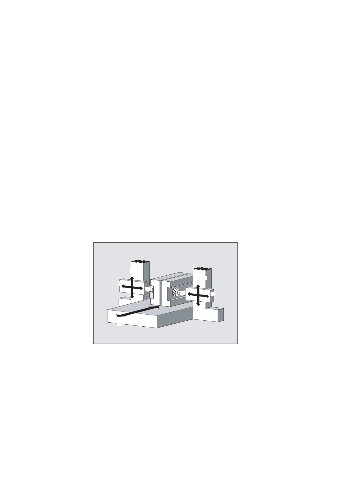
● Two-sided machining with 2 coupled motion groups:

1. Leading axis Y, coupled motion axis V

2. Leading axis Z, coupled motion axis W

$[LV

;

Syntax

TRAILON(<following axis>,<leading axis>,<coupling factor>)

TRAILOF(<following axis>,<leading axis>,<leading axis 2>)

TRAILOF(<following axis>)

Job Planning

Programming Manual, 03/2010, 6FC5398-2BP20-1BA0

497

Axis couplings

9.1 Coupled motion (TRAILON, TRAILOF)

Significance

TRAILON

Command for activating and defining a coupled axis grouping

Active:

modal

Parameter 1: Axis name of trailing axis

Note:

A coupled-motion axis can also act as the leading axis for other

coupled-motion axes. In this way, it is possible to create a range

of different coupled axis groupings.

Parameter 2: Axis name of trailing axis

Parameter 3: Coupling factor

The coupling factor specifies the desired relationship between the

paths of the coupled-motion axis and the leading axis:

<coupling factor> = path of coupled-motion axis/path of leading

axis

Type: REAL

Default:

The input of a negative value causes the master and coupled axes

to traverse in opposition.

If a coupling factor is not programmed, then coupling factor 1

automatically applies.

TRAILOF

Command for deactivating a coupled axis grouping

Effective:

modal

TRAILOF with 2 parameters deactivates only the coupling to the

specified leading axis:

TRAILOF(<following axis>,<leading axis>)

If a coupled-motion axis has 2 leading axes, TRAILOF can be called

with 3 parameters to deactivate both couplings.

TRAILOF(<following axis>,<leading axis>,<leading axis 2>)

Programming TRAILOF without specifying a leading axis produces the

same result:

TRAILOF(<following axis>)

Note

Coupled axis motion is always executed in the base coordinate system (BCS).

The number of coupled axis groupings which may be simultaneously activated is limited only

by the maximum possible number of combinations of axes on the machine.

Job Planning

498

Programming Manual, 03/2010, 6FC5398-2BP20-1BA0

Axis couplings

9.1 Coupled motion (TRAILON, TRAILOF)

Example

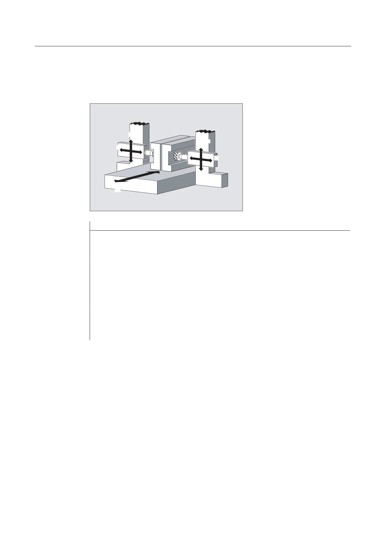
The workpiece is to be machined on two sides with the axis configuration shown in the

diagram. To do this, you create two combinations of coupled axes.

$[LV

;

Program code

Comments

…

N100 TRAILON(V,Y)

; Activation of 1st coupled axis grouping

N110 TRAILON(W,Z,-1)

; Activation of 2nd coupled axis grouping, Negative

coupling factor: Coupled-motion axis traverses in the

opposite direction from leading axis.

N120 G0 Z10

; Infeed of Z and W axes in opposite axial directions.

N130 G0 Y20

; Infeed of Y and V axes in same axis direction.

…

N200 G1 Y22 V25 F200

; Overlaying of a dependent and independent movement of

coupled motion axis V.

…

TRAILOF(V,Y)

; Deactivation of 1st coupled axis grouping.

TRAILOF(W,Z)

; Deactivation of 2nd coupled axis grouping.

Further Information

Axis types

A coupled axis grouping can consist of any desired combinations of linear and rotary axes. A

simulated axis can also be defined as a leading axis.

Coupled-motion axes

Up to two leading axes can be assigned simultaneously to a trailing axis. The assignment is

made in different combinations of coupled axes.

A coupled-motion axis can be programmed with the full range of available motion commands

(G0, G1, G2, G3, etc.). The coupled axis not only traverses the independently defined paths, but

also those derived from its leading axes on the basis of coupling factors.

Job Planning

Programming Manual, 03/2010, 6FC5398-2BP20-1BA0

499

Axis couplings

9.1 Coupled motion (TRAILON, TRAILOF)

Dynamics limit

The dynamics limit is dependent on the type of activation of the coupled axis grouping:

● Activation in part program

If activation is performed in the part program and all leading axes are active as program

axes in the activated channel, the dynamic response of all coupled-motion axes is taken

into account during traversing of the leading axis to avoid overloading the coupled-motion

axes.

If activation is performed in the part program with leading axes that are not active as

program axes in the activating channel ($AA_TYP ≠ 1), then the dynamic response of the

coupled-motion axes is not taken into account during traversing of the leading axis. This

can cause the overloading of coupled-motion axes with a dynamic response which is less

than that required for the coupling.

● Activation in synchronized action

If activation is performed in a synchronized action, the dynamic response of the coupled-

motion axes is not taken into account during traversing of the leading axis. This can

cause the overloading of coupled-motion axes with a dynamic response which is less

than that required for the coupling.

CAUTION

If a coupled axis grouping is activated:

• in synchronized actions

• in the part program with leading axes that are not program axes in the channel of the

coupled-motion axes

it is the specific responsibility of the user/machine manufacturer to take suitable action

to ensure that the traversing of the leading axis will not cause the overloading of the

coupled-motion axes.

Coupling status

The coupling status of an axis can be checked in the part program with the system variable:

$AA_COUP_ACT[<axis>]

Value

Significance

No coupling active

Coupled motion active

Job Planning

500

Programming Manual, 03/2010, 6FC5398-2BP20-1BA0

Axis couplings

9.2 Curve tables (CTAB)

9.2

Curve tables (CTAB)

Function

Curve tables can be used to program position and velocity relationships between two axes

(leading and following axis). Curve tables are defined in the part program.

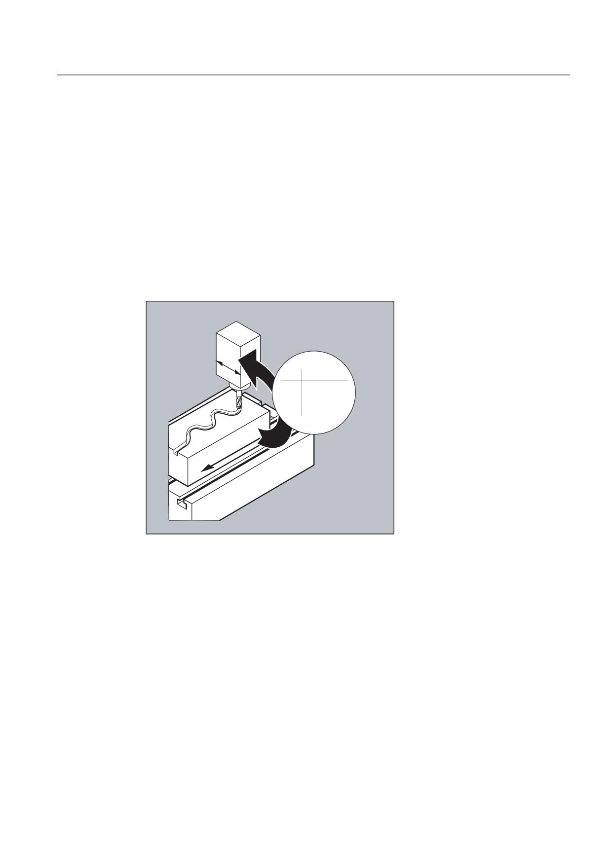
Application

Curve tables replace mechanical cams. The curve table forms the basis for the axial master

value coupling by creating the functional relationship between the leading and the following

value: With appropriate programming, the control calculates a polynomial that corresponds

to the cam from the relative positions of the leading and following axes.

[

D D D[

D D[

;

Job Planning

Programming Manual, 03/2010, 6FC5398-2BP20-1BA0

501

Axis couplings

9.2 Curve tables (CTAB)

9.2.1

Define curve tables (CTABDEF, CATBEND)

Function

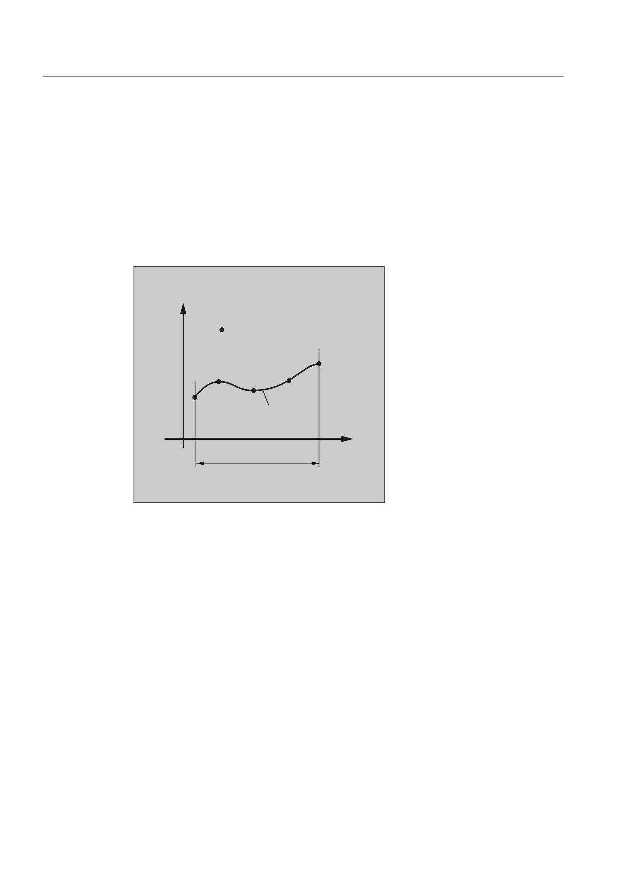
A curve table represents a part program or a section of a part program enclosed by CTABDEF

at the start and CTABEND at the end.

Within this part program section, unique following axis positions are assigned to individual

positions of the leading axis using motion operations; these following axis positions are used

as intermediate points when calculating the curve definition in the form of a polynomial up to

the 5th order.

6ODYH YDOXH

LQWHUPHGLDWH SRLQW

&XUYH WUDFH

0DVWHU YDOXH

'HILQLWLRQ UDQJH

6WDUWLQJ YDOXH

(QG YDOXH

Condition

The MD must be configured accordingly to ensure that sufficient memory space is reserved

for the definition of curve tables (→ machine manufacturer).

Syntax

CTABDEF(<following axis>,<leading axis>,<n>,<periodicity>[,<memory

location>])

CTABEND

Job Planning

502

Programming Manual, 03/2010, 6FC5398-2BP20-1BA0

Axis couplings

9.2 Curve tables (CTAB)

Significance

CTABDEF( )

Start of curve table definition

CTABEND

End of curve table definition

Axis whose motion is to be calculated using the curve table

Axis providing the master values for the calculation of the following

axis motion

<n>

Number (ID) of curve table

The number of a curve table is unique and independent of the

memory location. It is not possible for there to be tables with the

same number in the static and dynamic NC memory.

Table periodicity

Table is non-periodic (table is processed only once, even for

rotary axes)

Table is periodic with regard to the leading axis

Table is periodic with regard to leading axis and following axis

Specification of memory location (optional)

"SRAM"

The curve table is created in the static NC memory.

"DRAM"

The curve table is created in the dynamic NC memory.

Note:

If a value is not programmed for this parameter, the default memory

location set with

MD20905 $MC_CTAB_DEFAULT_MEMORY_TYPE is used.

Note

Overwrite

A curve table is overwritten as soon as its number (<n>) is used in another table definition

(exception: the curve table is in active in an axis coupling or locked with CTABLOCK). No

warning is output when curve tables are overwritten.

Job Planning

Programming Manual, 03/2010, 6FC5398-2BP20-1BA0

503

Axis couplings

9.2 Curve tables (CTAB)

Examples

Example 1: Program section as curve table definition

A program section is to be used unchanged for defining a curve table. The STOPRE command

for preprocessing stop can remain and is reactivated immediately as soon as the program

section is no longer being used for table definition and CTABDEF and CTABEND have been

removed.

Program code

Comments

…

CTABDEF(Y,X,1,1)

; Definition of a curve table.

…

IF NOT ($P_CTABDEF)

STOPRE

ENDIF

…

CTABEND

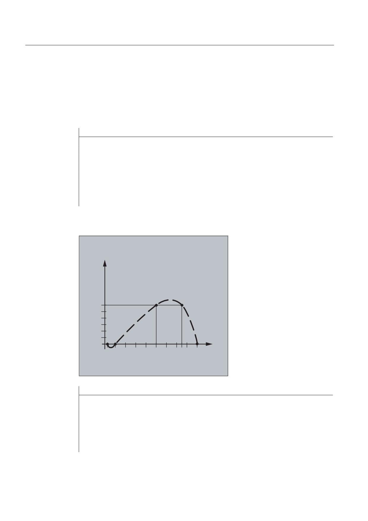
Example 2: Definition of a non-periodic curve table

;

Program code

Comments

N100 CTABDEF(Y,X,3,0)

; Beginning of the definition of a ;non-periodic curve

table with number 3.

N110 X0 Y0

; 1st motion operation, defines the starting values and

1st intermediate point:

Master value: 0, Following value: 0

N120 X20 Y0

; 2nd intermediate point

Master value: 0…20, Following value: starting value…0

Job Planning

504

Programming Manual, 03/2010, 6FC5398-2BP20-1BA0

Axis couplings

9.2 Curve tables (CTAB)

Program code

Comments

N130 X100 Y6

;

3rd intermediate point:

Master value: 20…100, Following value: 0 to 6

N140 X150 Y6

;

4th intermediate point:

Master value: 100…150, Following value: 6 to 6

N150 X180 Y0

;

5th intermediate point:

Master value: 150…180, Following value: 6 to 0

N200 CTABEND

; End of definition. The curve table is generated in

its internal representation as a polynomial of up to

the 5th order. The calculation of the curve

definition with the specified intermediate points is

dependent on the modally selected interpolation type

(circular, linear, spline interpolation). The part

program state before starting the definition is

restored.

Example 3: Definition of a periodic curve table

Definition of a periodic curve table with number 2, master value range 0 to 360, following

axis motion from 0 to 45 and back to 0:

Program code

Comments

N10 DEF REAL DEPPOS

N20 DEF REAL GRADIENT

N30 CTABDEF(Y,X,2,1)

; Start of definition

N40 G1 X=0 Y=0

N50 POLY

N60 PO[X]=(45.0)

N70 PO[X]=(90.0) PO[Y]=(45.0,135.0,-90)

N80 PO[X]=(270.0)

N90 PO[X]=(315.0) PO[Y]=(0.0,-135.0,90)

N100 PO[X]=(360.0)

N110 CTABEND

; End of definition

;Test of the curve by coupling Y to X:

N120 G1 F1000 X0

N130 LEADON(Y,X,2)

N140 X360

N150 X0

N160 LEADOF(Y,X)

N170 DEPPOS=CTAB(75.0,2,GRADIENT)

; Read the table function for

master value 75.0.

N180 G0 X75 Y=DEPPOS

; Positioning leading and following

axes.

;After activating the coupling, no synchronization of the following axis is

required.

N190 LEADON(Y,X,2)

N200 G1 X110 F1000

N210 LEADOF(Y,X)

N220 M30

Job Planning

Programming Manual, 03/2010, 6FC5398-2BP20-1BA0

505

Axis couplings

9.2 Curve tables (CTAB)

Further information

Starting and end value of the curve table

The starting value for the beginning of the definition range of the curve table are the first

associated axis positions specified (the first traverse statement) within the curve table

definition. The end value of the definition range of the curve table is determined in

accordance with the last traverse command.

Available language scope

Within the definition of the curve table, you have use of the entire NC language.

Note

The following entries are not permitted in curve table definitions:

• Preprocessing stop

• Jumps in the leading axis movement (e.g. on changing transformations)

• Traverse statement for the following axis only

• Reversal of the leading axis, i.e. position of the leading axis must always be unique

• CTABDEF and CTABEND operation on different program levels.

Effectiveness of modal operations

All modal statements that are made within the curve table definition are invalid when the

table definition is completed. The part program in which the table definition is made is

therefore before and after the table definition in the same state.

Assignments to R-parameters

Assignments to R-parameters in the table definition are reset after CTABEND.

Example:

Program code

Comments

R10=5 R11=20

; R10=5

CTABDEF

G1 X=10 Y=20 F1000

R10=R11+5

; R10=25

X=R10

CTABEND

; R10=5

Job Planning

506

Programming Manual, 03/2010, 6FC5398-2BP20-1BA0

Axis couplings

9.2 Curve tables (CTAB)

Activating ASPLINE, BSPLINE, CSPLINE

If an ASPLINE, BSPLINE or CSPLINE is activated within a curve table definition CTABDEF ...

CTABEND, at least one starting point should be programmed before this spline activation.

Immediate activation after CTABDEF should be avoided, otherwise the spline will depend on

the current axis position before the curve table definition.

Example:

Program code

CTABDEF(Y,X,1,0)

X0 Y0

ASPLINE

X=5 Y=10

X10 Y40

CTABEND

Repeated use of curve tables

The functional relationship between the leading axis and the following axis calculated using

the curve table will be retained under the selected table number after the end of the part

program and POWER OFF if the table has been saved to the static NC memory (SRAM).

A table created in the dynamic memory (DRAM) will be deleted on POWER ON and may

have to be regenerated.

Once created, the curve table can be applied to any axis combinations of leading and

following axis and is independent of the axes used to create the curve table.

Overwriting curve tables

A curve table is overwritten as soon as its number is used in another table definition.

Exception: A curve table is either active in an axis coupling or locked with CTABLOCK.

Note

No warning is output when curve tables are overwritten.

Curve table definition active?

The $P_CTABDEF system variable can be used at any time in the part program to check

whether a curve table definition is active.

Revoking the curve table definition

Once the operations relating to the curve table definition have been excluded, the part

program section can be used as a real part program again.

Job Planning

Programming Manual, 03/2010, 6FC5398-2BP20-1BA0

507

Axis couplings

9.2 Curve tables (CTAB)

Loading curve tables using "Execution from external source"

If curve tables are executed from an external source, the selection of the size of the reload

buffer (DRAM) in MD18360 $MN_MM_EXT_PROG_BUFFER_SIZE has to support the

simultaneous storage of the entire curve table definition in the reload buffer. If it is not, part

program processing will be canceled with an alarm.

Jumps in the following axis

Depending on the setting in machine data

MD20900 $MC_CTAB_ENABLE_NO_LEADMOTION,

jumps in the following axis may be tolerated if a movement is missing in the leading axis.

9.2.2

Check for presence of curve table (CTABEXISTS)

Function

The CTABEXISTS command can be used to check if a specific curve table number is present in

the NC memory.

Syntax

CTABEXISTS(<n>)

Significance

CTABEXISTS

Checks for the presence of curve table number <n> in the static or

dynamic NC memory.

Table does not exist

Table exists

<n>

Number (ID) of curve table

9.2.3

Delete curve tables (CTABDEL)

Function

CTABDEL can be used to delete curve tables.

Note

Curve tables that are active in an axis coupling cannot be deleted.

Job Planning

508

Programming Manual, 03/2010, 6FC5398-2BP20-1BA0

Axis couplings

9.2 Curve tables (CTAB)

Syntax

CTABDEL(<n>)

CTABDEL(<n>,<m>)

CTABDEL(<n>,<m>,<memory location>)

CTABDEL ()

CTABDEL(,,<memory location>)

Significance

CTABDEL

Command for deleting curve tables

<n>

Number (ID) of the curve table to be deleted

When a curve table range CTABDEL(<n>,<m>) is deleted, <n> is used

to specify the number of the first curve table in the range.

<m>

When a curve table range CTABDEL(<n>,<m>) is deleted, <m> is used

to specify the number of the last curve table in the range.

<m> has to be greater than <n>.

Specification of memory location (optional)

In the case of deletion without a memory location being specified,

the specified curve tables are deleted in the static and the dynamic

NC memory.

In the case of deletion with a memory location being specified, of the

specified curve tables, only those located in the specified memory

location are deleted. The rest are retained.

"SRAM"

Deletion in the static NC memory

"DRAM"

Deletion in the dynamic NC memory

If CTABDEL is programmed without specification of the curve table to be deleted, then all curve

tables or all curve tables in the specified memory will be deleted:

CTABDEL ()

Deletes all curve tables in the static and the dynamic NC

memory

CTABDEL(,,"SRAM")

Deletes all curve tables in the static NC memory

CTABDEL(,,"DRAM")

Deletes all curve tables in the dynamic NC memory

Note

If, in the case of multiple deletion with CTABDEL(<n>,<m>) or CTABDEL(), at least one of the of

the curve tables to be deleted is active in a coupling, the delete command will not be

executed; in other words, none of the addressed curve tables will be deleted.

Job Planning

Programming Manual, 03/2010, 6FC5398-2BP20-1BA0

509

Axis couplings

9.2 Curve tables (CTAB)

9.2.4

Locking curve tables to prevent deletion and overwriting (CTABLOCK,

CTABUNLOCK)

Function

Locks can be set to protect curve tables against unintentional deletion and overwriting. Once

a lock has been set, it can be revoked at any time.

Syntax

Lock:

CTABLOCK(<n>)

CTABLOCK(<n>,<m>)

CTABLOCK(<n>,<m>,<memory location>)

CTABLOCK()

CTABLOCK(,,<memory location>)

Unlock:

CTABUNLOCK(<n>)

CTABUNLOCK(<n>,<m>)

CTABUNLOCK(<n>,<m>,<memory location>)

CTABUNLOCK()

CTABUNLOCK(,,<memory location>)

Significance

CTABLOCK

Command for setting a lock to prevent deletion/overwriting

CTABUNLOCK

Command for revoking a lock to prevent deletion/overwriting

CTABUNLOCK unlocks the curve tables locked with CTABLOCK. Curve

tables which are involved in an active coupling remain locked and

cannot be deleted. The lock with CTABLOCK is unlocked as soon as

the lock applied due to the active coupling is unlocked when the

coupling is deactivated. This table can therefore be deleted. It is not

necessary to call CTABUNLOCK again.

<n>

Number (ID) of the curve table to be locked/unlocked

When a curve table range CTABLOCK(<n>,<m>)/CTABUNLOCK(<n>,<m>) is

locked/unlocked, <n> is used to specify the number of the first curve

table in the range.

Job Planning

510

Programming Manual, 03/2010, 6FC5398-2BP20-1BA0

Axis couplings

9.2 Curve tables (CTAB)

<m>

When a curve table range CTABLOCK(<n>,<m>)/CTABUNLOCK(<n>,<m>) is

locked/unlocked, <m> is used to specify the number of the last curve

table in the range.

<m> has to be greater than <n>.

Specification of memory location (optional)

In the case of locking/unlocking without a memory location being

specified, the specified curve tables are locked/unlocked in the static

and the dynamic NC memory.

In the case of locking/unlocking with a memory location being

specified, of the specified curve tables, only those located in the

specified memory location are locked/unlocked. The rest are not

locked/unlocked.

"SRAM"

Lock/unlock in the static NC memory

"DRAM"

Lock/unlock in the dynamic NC memory

If CTABLOCK/CTABUNLOCK is programmed without specification of the curve table to be

locked/unlocked, then all curve tables or all curve tables in the specified memory will be

locked/unlocked:

CTABLOCK()

Locks all curve tables in the static and the dynamic NC

memory

CTABLOCK(,,"SRAM")

Locks all curve tables in the static NC memory

CTABLOCK(,,"DRAM")

Locks all curve tables in the dynamic NC memory

CTABUNLOCK()

Unlocks all curve tables in the static and dynamic NC

memory

CTABUNLOCK(,,"SRAM")

Unlocks all curve tables in the static NC memory

CTABUNLOCK(,,"DRAM")

Unlocks all curve tables in the dynamic NC memory

9.2.5

Curve tables: Determine table properties (CTABID, CTABISLOCK,

CTABMEMTYP, CTABPERIOD)

Function

These commands can be used to poll important properties of a curve table (table number,

lock state, memory location, periodicity).

Syntax

CTABID()

CTABID(,<memory location>)

CTABISLOCK(<n>)

CTABMEMTYP(<n>)

TABPERIOD(<n>)

Job Planning

Programming Manual, 03/2010, 6FC5398-2BP20-1BA0

511

Axis couplings

9.2 Curve tables (CTAB)

Significance

CTABID

Returns the table number entered as the th curve table in the

specified memory.

Example:

CTABID(1,"SRAM") returns the number of the first curve table in the

static NC memory. In this context the first curve table is the curve

table with the highest table number.

Note:

If the sequence of curve tables in the memory changes between

consecutive calls of CTABID, e.g. due to the deletion of curve tables

with CTABDEL, CTABID(,...) can return a different curve table with

the same number .

CTABISLOCK

Returns the lock state of curve table number <n>:

Table is not locked

Table is locked by CTABLOCK

Table is locked by active coupling

Table is locked by CTABLOCK and active coupling

-1

Table does not exist

CTABMEMTYP

Returns the memory location of curve table number <n>:

Table in the static NC memory

Table in the dynamic NC memory

-1

Table does not exist

CTABPERIOD

Returns the periodicity of curve table number <n>:

Table is not periodic

Table is periodic in the leading axis

Table is periodic in the leading and following axes

-1

Table does not exist

Entry number in memory

<n>

Number (ID) of curve table

Specification of memory location (optional)

"SRAM"

Static NC memory

"DRAM"

Dynamic NC memory

Note:

If a value is not programmed for this parameter, the default memory

location set with

MD20905 $MC_CTAB_DEFAULT_MEMORY_TYPE is used.

Job Planning

512

Programming Manual, 03/2010, 6FC5398-2BP20-1BA0

Axis couplings

9.2 Curve tables (CTAB)

9.2.6

Read curve table values (CTABTSV, CTABTEV, CTABTSP, CTABTEP,

CTABSSV, CTABSEV, CTAB, CTABINV, CTABTMIN, CTABTMAX)

Function

The following curve table values can be read in the part program:

● Following axis and leading axis values at the start and end of a curve table

● Following axis values at the start and end of a curve segment

● Following axis value for a leading axis value

● Leading axis value for a following axis value

● Following axis minimum and maximum values

- In the entire definition range of the curve table

- In a defined curve table interval

Syntax

CTABTSV(<n>,<gradient>[,<following axis>])

CTABTEV(<n>,<gradient>[,<following axis>])

CTABTSP(<n>,<gradient>[,<leading axis>])

CTABTEP(<n>,<gradient>[,<leading axis>])

CTABSSV(<master value>,<n>,<gradient>[,<following axis>])

CTABSEV(<master value>,<n>,<gradient>[,<following axis>])

CTAB(<master value>,<n>,<gradient>[,<following axis>,<leading axis>]

CTABINV(<following value>,<approximate

value>,<n>,<gradient>[,<following axis>,<leading axis>]

CTABTMIN(<n>[,<following axis>])

CTABTMAX(<n>[,<following axis>])

CTABTMIN(<n>,<a>,[,<following axis>,<leading axis>])

CTABTMAX(<n>,<a>,[,<following axis>,<leading axis>])

Job Planning

Programming Manual, 03/2010, 6FC5398-2BP20-1BA0

513

Axis couplings

9.2 Curve tables (CTAB)

Meaning

CTABTSV:

Read following axis value at the start of curve table no. <n>

CTABTEV:

Read following axis value at the end of curve table no. <n>

CTABTSP:

Read leading axis value at the start of curve table no. <n>

CTABTEP:

Read leading axis value at the end of curve table no. <n>

CTABSSV:

Read following axis value at the start of the curve segment

belonging to the specified leading axis value (<master value>)

CTABSEV:

Read following axis value at the end of the curve segment

belonging to the specified leading axis value (<master value>)

CTAB:

Read following axis value for specified leading axis value (<master

value>)

CTABINV:

Read leading axis value for specified following axis value

(<following value>)

CTABTMIN:

Define following axis minimum value:

• In the entire definition range of the curve table

• In a defined interval <a> to

CTABTMAX:

Define following axis maximum value:

• In the entire definition range of the curve table

• In a defined interval <a> to

<n>:

Number (ID) of curve table

<gradient>:

The <gradient> parameter returns the incline of the curve table

function at the calculated position.

<following axis>:

Axis whose motion is to be calculated using the curve table

(optional)

<leasing axis>:

Axis providing the master values for the calculation of the following

axis motion (optional)

<following value>:

Following axis value for reading the associated leading axis value

for CTABINV

<leading value>:

Leading axis value:

• for reading the associated following axis value with CTAB

• for the selection of the curve segment with CTABSSV/CTABSEV

<approximate value>:

The assignment of a leading axis value to a following axis value

with CTABINV must not always be unique. CTABINV requires,

therefore, an approximate value for the expected leading axis

value as a parameter.

<a>:

Lower limit of the master value interval with CTABTMIN/CTABTMAX

:

Upper limit of the master value interval with CTABTMIN/CTABTMAX

Note:

The master value interval <a> to always has to be within the

curve table's definition range.

Job Planning

514

Programming Manual, 03/2010, 6FC5398-2BP20-1BA0

Axis couplings

9.2 Curve tables (CTAB)

Examples

Example 1:

Define following axis and leading axis values at the start and end of the curve table, along

with the minimum and maximum values of the following axis in the entire definition range of

the curve table.

Program code

Comment

N10 DEF REAL STARTPOS

N20 DEF REAL ENDPOS

N30 DEF REAL STARTPARA

N40 DEF REAL ENDPARA

N50 DEF REAL MINVAL

N60 DEF REAL MAXVAL

N70 DEF REAL GRADIENT

N100 CTABDEF(Y,X,1,0)

; Beginning of table definition

N110 X0 Y10

; Start position 1st table segment

N120 X30 Y40

; End position 1st table segment = start position 2nd

table segment

N130 X60 Y5

; End position 2nd table segment = etc.

N140 X70 Y30

N150 X80 Y20

N160 CTABEND

; End of table definition.

N200 STARTPOS=CTABTSV(1,GRADIENT)

; Following axis value at start of curve table = 10

N210 ENDPOS=CTABTEV(1,GRADIENT)

; Following axis value at end of curve table = 20

N220 STARTPARA=CTABTSP(1,GRADIENT)

; Leading axis value at start of curve table = 0

N230 ENDPARA=CTABTEP(1,GRADIENT)

; Leading axis value at end of curve table = 80

N240 MINVAL=CTABTMIN(1)

; Minimum value of following axis with Y=5

N250 MAXVAL=CTABTMAX(1)

; Maximum value of following axis with Y=40

Example 2:

Determination of following axis values at the start and end of the curve segment associated

with leading axis value X=30.

Program code

Comment

N10 DEF REAL STARTPOS

N20 DEF REAL ENDPOS

N30 DEF REAL GRADIENT

N100 CTABDEF(Y,X,1,0)

; Beginning of table definition

N110 X0 Y0

; Start position 1st table segment

N120 X20 Y10

; End position 1st table segment = start position 2nd

table segment

Job Planning

Programming Manual, 03/2010, 6FC5398-2BP20-1BA0

515

Axis couplings

9.2 Curve tables (CTAB)

Program code

Comment

N130 X40 Y40

End position 2nd table segment = etc.

N140 X60 Y10

N150 X80 Y0

N160 CTABEND

; End of table definition.

N200 STARTPOS=CTABSSV(30.0,1,GRADIENT)

; Start position Y in 2nd segment = 10

N210 ENDPOS=CTABSEV(30.0,1,GRADIENT)

; End position Y in 2nd segment = 40

Further information

Use in synchronized actions

All commands for reading curve table values can also be used in synchronized actions (see

also the chapter titled "Motion-synchronous actions").

When using the CTABINV, CTABTMIN, and CTABTMAX commands, make sure that:

● Sufficient NC power is available at the time of execution

● The number of segments in the curve table is queried prior to the call, so that the table

concerned can be subdivided if necessary

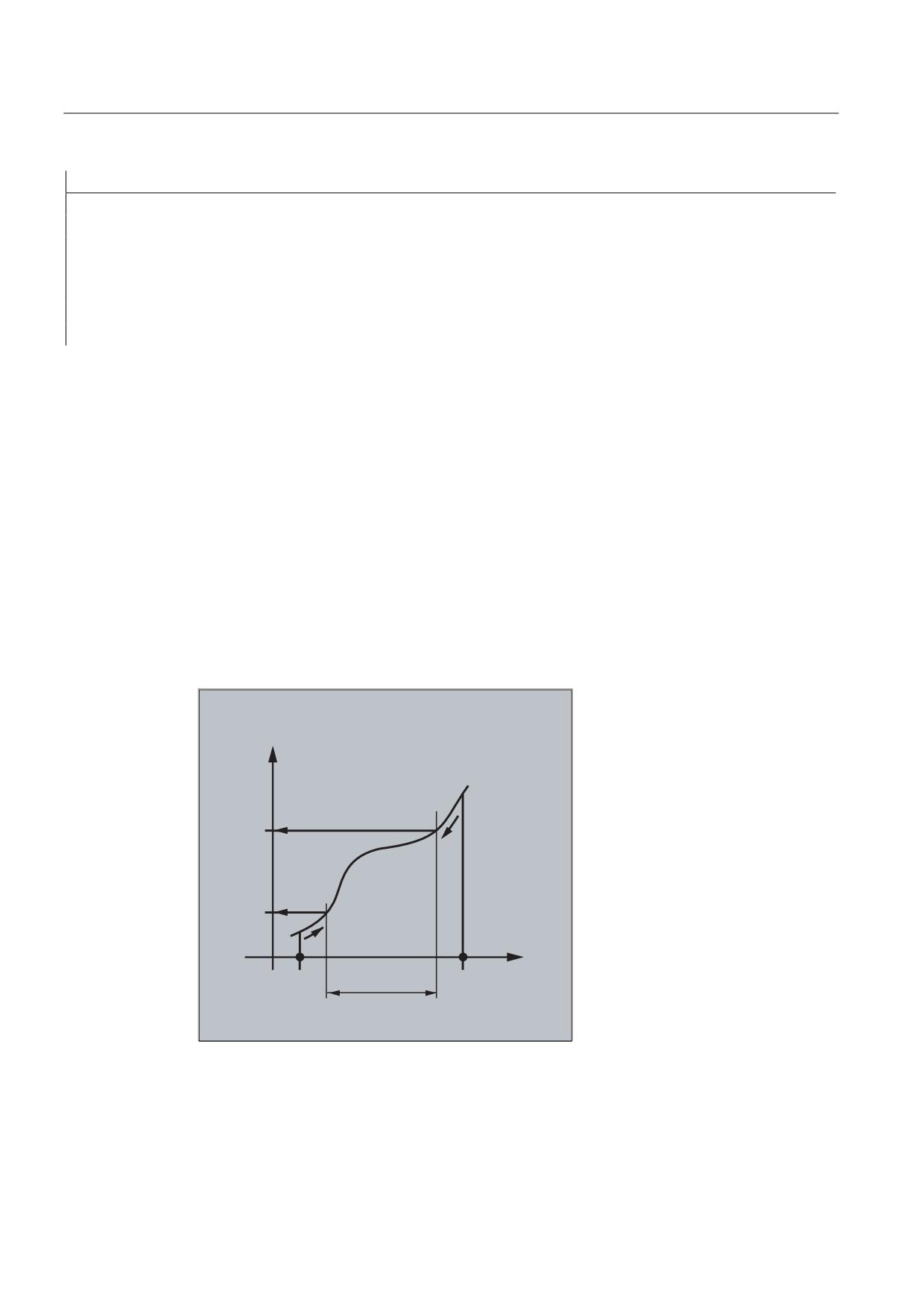
CTAB with non-periodic curve tables

If the specified <master value> is outside the definition range, the upper or lower limit will be

output as the following value:

6ODYH YDOXH

)

0DVWHU

'HILQLWLRQ UDQJH

YDOXH

Job Planning

516

Programming Manual, 03/2010, 6FC5398-2BP20-1BA0

Axis couplings

9.2 Curve tables (CTAB)

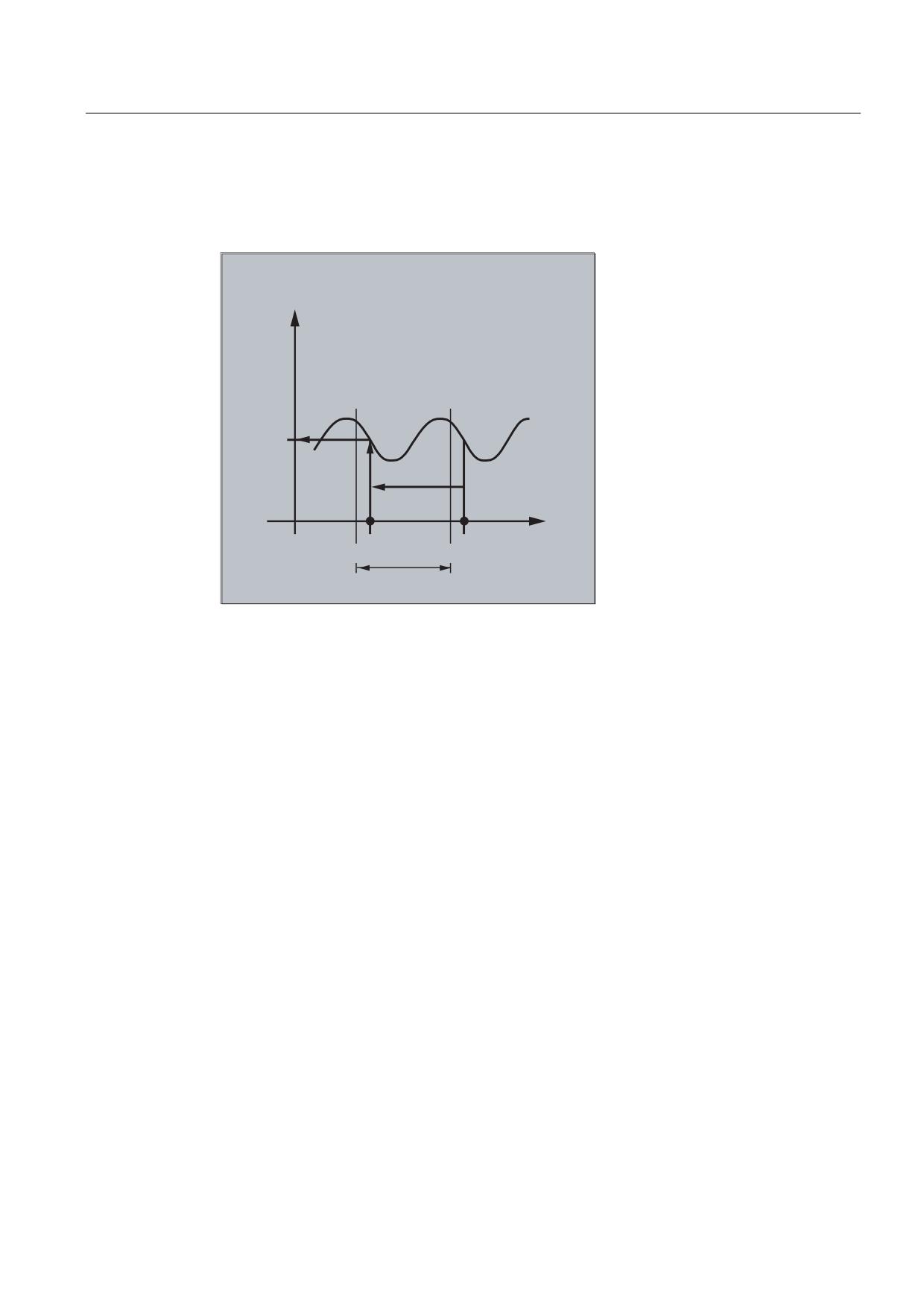
CTAB with periodic curve tables

If the specified <master value> is outside the definition range, the master value is evaluated

modulo of the definition range and the corresponding following value is output:

6ODYH YDOXH

)

0DVWHU

'HILQLWLRQ UDQJH

YDOXH

Approximate value for CTABINV

The CTABINV command, therefore, requires an approximate value for the expected master

value. CTABINV returns the master value that is closest to the approximate value. The

approximate value can be, for example, the master value from the previous interpolation

cycle.

Incline of the curve table function

The output of the incline (<gradient>) makes it possible to calculate the velocity of the

leading or following axis at the corresponding position.

Specification of the leading or following axis

The optional specification of the leading and/or following axis is important if the leading and

following axes are configured in different length units.

CTABSSV, CTABSEV

The CTABSSV and CTABSEV commands are not suitable to query programmed segments in the

following cases:

● Circles or involutes are programmed.

● Chamfer or rounding with CHF/ RND is active

● Smoothing with G643 is active

● NC block compression with COMPON/COMPCURV/COMPCAD is active

Job Planning

Programming Manual, 03/2010, 6FC5398-2BP20-1BA0

517

Axis couplings

9.2 Curve tables (CTAB)

9.2.7

Curve tables: Check use of resources (CTABNO, CTABNOMEM, CTABFNO,

CTABSEGID, CTABSEG, CTABFSEG, CTABMSEG, CTABPOLID, CTABPOL,

CTABFPOL, CTABMPOL)

Function

The programmer can use these commands to obtain up-to-date information about the use of

resources for curve tables, table segments, and polynomials.

Syntax

CTABNO

CTABNOMEM(<memory location>)

CTABFNO(<memory location>)

CTABSEGID(<n>,<memory location>)

CTABSEG(<memory location>,<segment type>)

CTABFSEG(<memory location>,<segment type>)

CTABMSEG(<memory location>,<segment type>)

CTABPOLID(<n>)

CTABPOL(<memory location>)

CTABFPOL(<memory location>)

CTABMPOL(<memory location>)

Significance

CTABNO

Determine total number of defined curve tables (in the static and the

dynamic NC memory)

CTABNOMEM

Determine the number of defined curve tables in the specified

CTABFNO

Determine the number of curve tables remaining possible in the

specified <memory location>

CTABSEGID

Determine the number of curve segments of the specified <segment

type> used by curve table number <n>

CTABSEG

Determine the number of curve segments of the specified <segment

type>used in the specified <memory location>

CTABFSEG

Determine the number of curve segments of the specified <segment

type> remaining possible in the specified <memory location>

CTABMSEG

Determine the maximum possible number of curve segments of the

specified <segment type> in the specified <memory location>

CTABPOLID

Determine the number of curve polynomials used by curve table

number <n>

CTABPOL

Determine the number of curve polynomials used in the specified

CTABFPOL

Determine the number of curve polynomials remaining possible in

the specified <memory location>

Job Planning

518

Programming Manual, 03/2010, 6FC5398-2BP20-1BA0

Axis couplings

9.2 Curve tables (CTAB)

CTABMPOL

Determine the maximum possible number of curve polynomials in

the specified <memory location>

<n>

Number (ID) of curve table

Specification of memory location (optional)

"SRAM"

Static NC memory

"DRAM"

Dynamic NC memory

Note:

If a value is not programmed for this parameter, the default memory

location set with

MD20905 $MC_CTAB_DEFAULT_MEMORY_TYPE is used.

Specification of segment type (optional)

"L"

Linear segments

"P"

Polynomial segments

Note:

If no value is programmed for this parameter, the sum of the linear

and polynomial segments is output.

Job Planning

Programming Manual, 03/2010, 6FC5398-2BP20-1BA0

519

Axis couplings

9.3 Axial leading value coupling (LEADON, LEADOF)

9.3

Axial leading value coupling (LEADON, LEADOF)

Note

This function is not available for SINUMERIK 828D!

Function

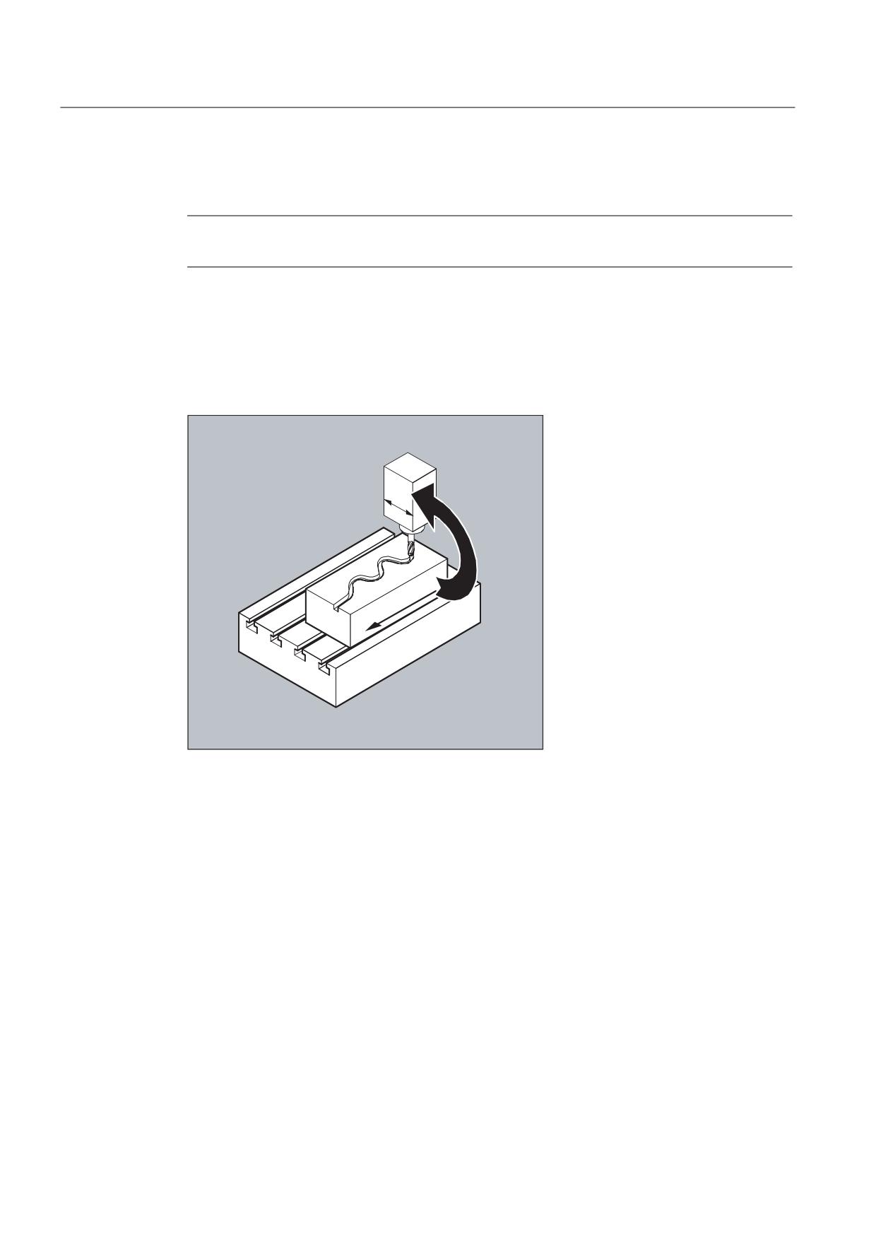
With the axial master value coupling, a leading and a following axis are moved in

synchronism. It is possible to assign the position of the following axis via a curve table or the

resulting polynomial uniquely to a position of the leading axis - simulated if necessary.

;

The leading axis is the axis which supplies the input values for the curve table. The following

axis is the axis, which takes the positions calculated by means of the curve table.

Actual value and setpoint coupling

The following can be used as the master value, i.e., as the output values for position

calculation of the following axis:

● Actual values of the leading axis position: Actual value coupling

● Setpoints of the leading axis position: Setpoint value coupling

The master value coupling always applies in the basic coordinate system.

For the creation of curve tables, see section "Curve tables".

For the master value coupling, see /FB/, M3, Coupled-axis motion and master value

coupling.

Job Planning

520

Programming Manual, 03/2010, 6FC5398-2BP20-1BA0

Axis couplings

9.3 Axial leading value coupling (LEADON, LEADOF)

Syntax

LEADON(FAxis,LAxis,n)

LEADOF(FAxis,LAxis)

or deactivation without specifying the leading axis:

LEADOF(FAxis)

The master value coupling can be activated and deactivated both from the part program and

during the movement from synchronized actions, see section "Motion synchronous actions" .

Significance

LEADON

Activate master value coupling

LEADOF

Deactivate master value coupling

Faxis

Following axis

Laxis

Leading axis

Curve table number

$SA_LEAD_TYPE

Switching between setpoint and actual value coupling

Deactivate master value coupling, LEADOF

When you deactivate the master value coupling, the following axis becomes a normal

command axis again!

Axial master value coupling and different operating states, RESET

Depending on the setting in the machine data, the master value couplings are deactivated

with RESET.

Example of master value coupling from synchronous action

In a pressing plant, an ordinary mechanical coupling between a leading axis (stanchion

shaft) and axis of a transfer system comprising transfer axes and auxiliary axes is to be

replaced by an electronic coupling system.

It demonstrates how a mechanical transfer system is replaced by an electronic transfer

system. The coupling and decoupling processes are implemented as static synchronized

actions.

From the leading axis LV (stanchion shaft), transfer axes and auxiliary axes are controlled as

following axes that are defined via curve tables.

Following axes

X feed or master value axis

YL closing or transverse axis

ZL lifting axis

U roll feed, auxiliary axis

V guide head, auxiliary axis

W greasing, auxiliary axis

Job Planning

Programming Manual, 03/2010, 6FC5398-2BP20-1BA0

521

Axis couplings

9.3 Axial leading value coupling (LEADON, LEADOF)

Actions

The actions that occur include, for example, the following synchronized actions:

● Activate coupling, LEADON(following axis, leading axis, curve table number)

● Deactivate coupling, LEADOF(following axis, leading axis)

● Set actual value, PRESETON(axis, value)

● Set marker, $AC_MARKER[i]= value

● Coupling type: real/virtual master value

● Approaching axis positions, POS[axis]=value

Conditions

Fast digital inputs, real-time variables $AC_MARKER and position comparisons are linked using

the Boolean operator AND for evaluation as conditions.

Note

In the following example, line change, indentation and bold type are used for the sole

purpose of improving readability of the program. To the control, everything that follows a line

number constitutes a single line.

Comments

Program code

Comments

; Defines all static synchronized actions.

;

****Reset marker

N2 $AC_MARKER[0]=0 $AC_MARKER[1]=0 $AC_MARKER[2]=0 $AC_MARKER[3]=0 $AC_MARKER[4]=0 $AC_MARKER[5]=0

$AC_MARKER[6]=0 $AC_MARKER[7]=0

;

**** E1 0=>1 transfer ON

N10 IDS=1 EVERY ($A_IN[1]==1) AND ($A_IN[16]==1) AND ($AC_MARKER[0]==0)

DO LEADON(X,LW,1) LEADON(YL,LW,2) LEADON(ZL,LW,3) $AC_MARKER[0]=1

;

**** E1 0=>1 coupling roller feed ON

N20 IDS=11 EVERY ($A_IN[1]==1) AND ($A_IN[5]==0) AND ($AC_MARKER[5]==0)

DO LEADON(U,LW,4) PRESETON(U,0) $AC_MARKER[5]=1

;

**** E1 0->1 coupling alignment head ON

N21 IDS=12 EVERY ($A_IN[1]==1) AND ($A_IN[5]==0) AND ($AC_MARKER[6]==0)

DO LEADON(V,LW,4) PRESETON(V,0) $AC_MARKER[6]=1

;

**** E1 0->1 lubrication coupling ON

N22 IDS=13 EVERY ($A_IN[1]==1) AND ($A_IN[5]==0) AND ($AC_MARKER[7]==0)

DO LEADON(W,LW,4) PRESETON(W,0) $AC_MARKER[7]=1

;

**** E2 0=>1 coupling OFF

N30 IDS=3 EVERY ($A_IN[2]==1)

DO LEADOF(X,LW) LEADOF(YL,LW) LEADOF(ZL,LW) LEADOF(U,LW) LEADOF(V,LW) LEADOF(W,LW) $AC_MARKER[0]=0

$AC_MARKER[1]=0 $AC_MARKER[3]=0 $AC_MARKER[4]=0 $AC_MARKER[5]=0 $AC_MARKER[6]=0 $AC_MARKER[7]=0

N110 G04 F01

N120 M30

Job Planning

522

Programming Manual, 03/2010, 6FC5398-2BP20-1BA0

Axis couplings

9.3 Axial leading value coupling (LEADON, LEADOF)

Description

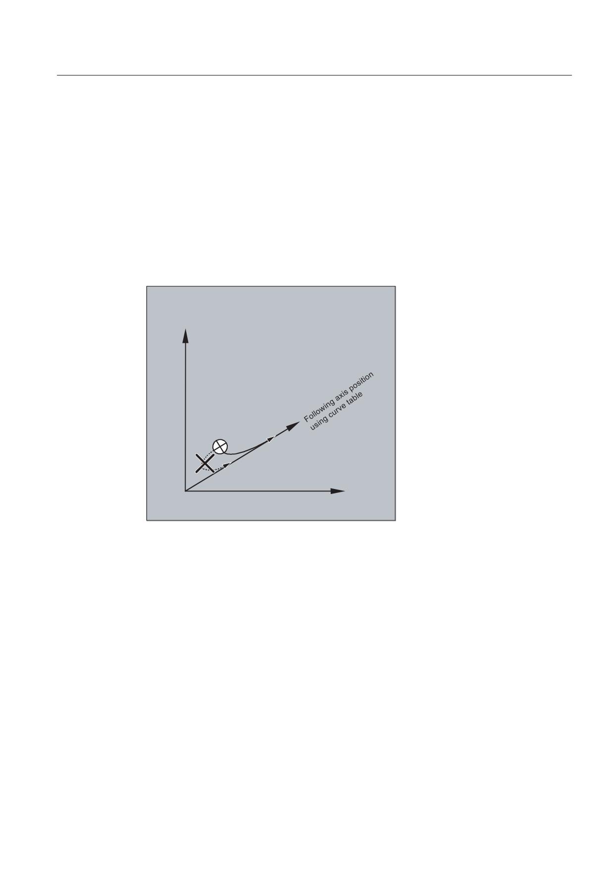
Master value coupling requires synchronization of the leading and the following axes. This

synchronization can only be achieved if the following axis is inside the tolerance range of the

curve definition calculated from the curve table when the master value coupling is activated.

The tolerance range for the position of the following axis is defined via machine data MD

37200: COUPLE_POS_POL_COARSE A_LEAD_TYPE.

If the following axis is not yet at the correct position when the master value coupling is

activated, the synchronization run is automatically initiated as soon as the position setpoint

value calculated for the following axis is approximately the real following axis position. During

the synchronization procedure the following axis is traversed in the direction that is defined

by the setpoint speed of the following axis (calculated from master spindle and using the

CTAB curve table).

)ROORZLQJ D[LV SRVLWLRQ

No synchronism

If the following axis position calculated moves away from the current following axis position

when the master value coupling is activated, it is not possible to establish synchronization.

Job Planning

Programming Manual, 03/2010, 6FC5398-2BP20-1BA0

523

Axis couplings

9.3 Axial leading value coupling (LEADON, LEADOF)

Actual value and setpoint coupling

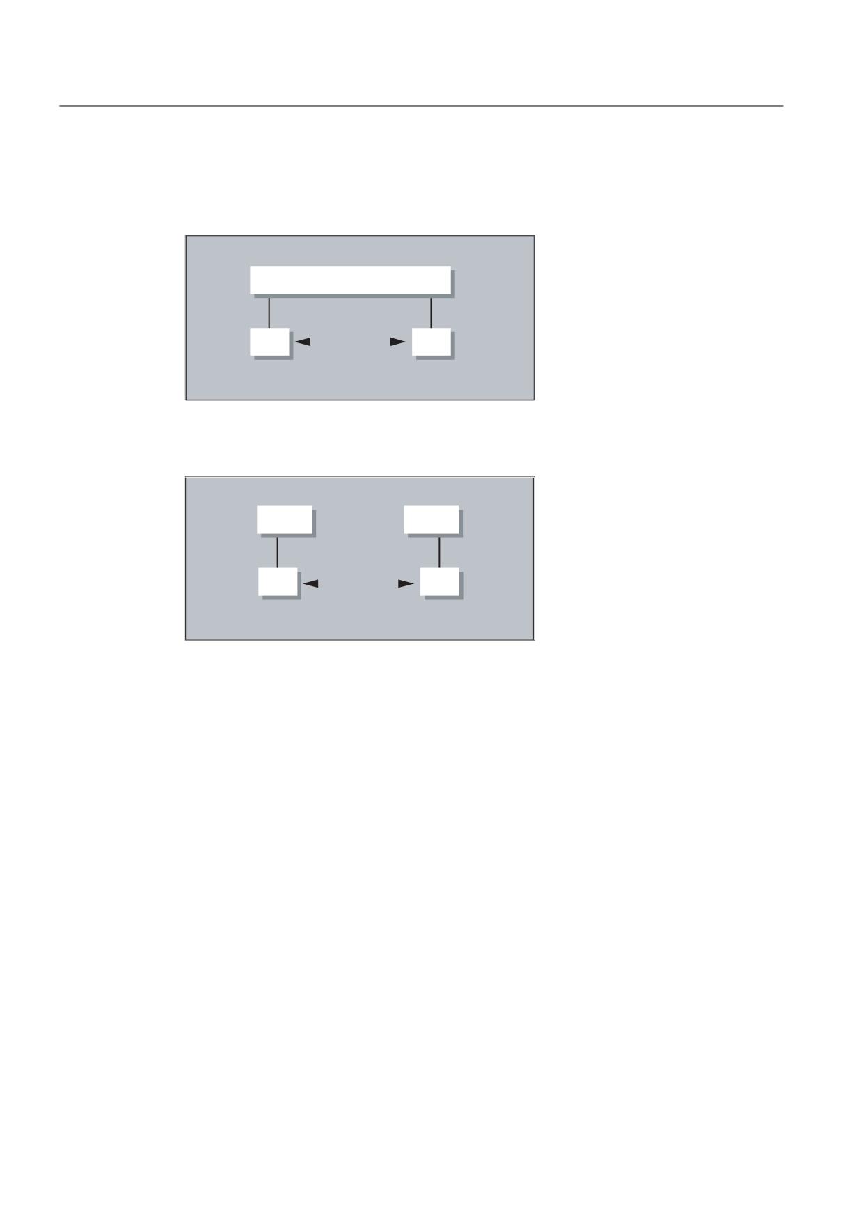
Setpoint coupling provides better synchronization of the leading and following axis than

actual value coupling and is therefore set by default.

1&8

6HWSRLQW YDOXH FRXSOLQJ

$FWXDO YDOXH FRXSOLQJ

Setpoint coupling is only possible if the leading and following axis are interpolated by the

same NCU. With an external leading axis, the following axis can only be coupled to the

leading axis via the actual values.

1&8

$FWXDO YDOXH FRXSOLQJ

A switchover can be programmed via setting data $SA_LEAD_TYPE

You must always switch between the actual-value and setpoint coupling when the following

axis stops. It is only possible to resynchronize after switchover when the axis is motionless.

Application example

You cannot read the actual values without error during large machine vibrations. If you use

master value coupling in press transfer, it might be necessary to switchover from actual-

value coupling to setpoint coupling in the work steps with the greatest vibrations.

Job Planning

524

Programming Manual, 03/2010, 6FC5398-2BP20-1BA0

Axis couplings

9.3 Axial leading value coupling (LEADON, LEADOF)

Master value simulation with setpoint coupling

Via machine data, you can disconnect the interpolator for the leading axis from the servo. In

this way you can generate setpoints for setpoint coupling without actually moving the leading

axis.

Master values generated from a setpoint link can be read from the following variables so that

they can be used, for example, in synchronized actions:

- $AA_LEAD_P

Master value position

- $AA_LEAD_V

Master value velocity

Create master value

As an option, master values can be generated with other self-programmed methods. The

master values generated in this way are written to and read from variables

- $AA_LEAD_SP

Master value position

- $AA_LEAD_SV

Master value velocity

Before you use these variables, the setting data $SA_LEAD_TYPE = 2 must be set.

Status of coupling

You can query the status of the coupling in the NC program with the following system

variable:

$AA_COUP_ACT[[axis]]

0: No coupling active

16: Master value coupling active

Status management for synchronized actions

Switching and coupling events are managed via real-time variables:

$AC_MARKER[i] = n

managed with:

i flag number

n status value

Job Planning

Programming Manual, 03/2010, 6FC5398-2BP20-1BA0

525

Axis couplings

9.4 Electronic gear (EG)

9.4

Electronic gear (EG)

Function

The "Electronic gear" function allows you to control the movement of a following axis

according to linear traversing block as a function of up to five leading axes. The relationship

between each leading axis and the following axis is defined by the coupling factor.

The following axis motion part is calculated by an addition of the individual leading axis

motion parts multiplied by their respective coupling factors. When an EG axis grouping is

activated, it is possible to synchronize the following axes in relation to a defined position. A

gear group can be:

● defined,

● activated,

● deactivated,

● deleted.

The following axis movement can be optionally derived from

● Setpoints of the leading axes, as well as

● Actual values of leading axes.

Non-linear relationships between each leading axis and the following axis can also be

realized as extension using curve tables (see "Path traversing behavior" section). Electronic

gears can be cascaded, i.e., the following axis of an electronic gear can be the leading axis

for a further electronic gear.

9.4.1

Defining an electronic gear (EGDEF)

Function

An EG axis group is defined by specifying the following axis and at least one, however not

more than five, leading axis, each with the relevant coupling type.

Requirements

Prerequisites for defining an EG axis group:

It is not permissible to define an axis coupling for the following axis (or an existing one must

first be deleted with EGDEL).

Syntax

EGDEF(following axis,leading axis1,coupling type1,leading

axis2,coupling type2,...)

Job Planning

526

Programming Manual, 03/2010, 6FC5398-2BP20-1BA0

Axis couplings

9.4 Electronic gear (EG)

Significance

EGDEF

Definition of an electronic gear

Following axis

Axis that is influenced by the leading axes

Leading axis1

,...,

Axes that influence the following axis

Leading axis5

Coupling type1

,...,

Coupling type

Coupling type5

The coupling type does not need to be the same for all leading

axes and must be programmed separately for each individual

master.

Value:

Significance:

The following axis is influenced by the actual value of

the corresponding leading axis.

The following axis is influenced by the setpoint of the

corresponding leading axis.

Note

The coupling factors are preset to zero when the EG axis grouping is defined.

Note

EGDEF triggers preprocessing stop. The gearbox definition with EGDEF should also be used

unaltered if, for systems, one or more leading axes affect the following axis via a curve table.

Example

Program code

Comments

EGDEF(C,B,1,Z,1,Y,1)

; Definition of an EG axis group. Leading axes B, Z, Y

influence the following axis C via the setpoint.

Job Planning

Programming Manual, 03/2010, 6FC5398-2BP20-1BA0

527

Axis couplings

9.4 Electronic gear (EG)

9.4.2

Switch-in the electronic gearbox (EGON, EGONSYN, EGONSYNE)

Function

There are 3 ways to switch-in an EG axis group.

Syntax

Variant 1:

The EG axis group is selectively switched-in without synchronization with:

EGON(FA,"block change mode",LA1,Z1,N1,LA2,Z2,N2,...,LA5,Z5,N5)

Variant 2:

The EG axis group is selectively activated with synchronization with:

EGONSYN(FA,"block change mode",SynPosFA,[,LAi,SynPosLAi,Zi,Ni])

Variant 3:

The EG axis group is selectively switched-in with synchronization and the approach mode

specified with:

EGONSYNE(FA,"block change mode",SynPosFA,approach

mode[,LAi,SynPosLAi,Zi,Ni])

Significance

Version 1:

Following axis

Block change mode

The following modes can be used:

"NOC"

Block change takes place immediately

"FINE"

Block change is performed in "Fine

synchronism"

"COARSE"

Block change is performed in "Coarse

synchronism"

"IPOSTOP"

Block change is performed for setpoint-

based synchronism

LA1, ... LA5

Leading axes

Z1, ... Z5

Counter for coupling factor i

N1, ... N5

Denominator for coupling factor i

Coupling factor i = Counter i / Denominator i

Only the leading axes previously specified with the EGDEF command may be programmed in

the activation line. At least one leading axis must be programmed.

Job Planning

528

Programming Manual, 03/2010, 6FC5398-2BP20-1BA0

Axis couplings

9.4 Electronic gear (EG)

Version 2:

Following axis

Block change mode

The following modes can be used:

"NOC"

Block change takes place immediately

"FINE"

Block change is performed in "Fine

synchronism"

"COARSE"

Block change is performed in "Coarse

synchronism"

"IPOSTOP"

Block change is performed for

setpoint-based synchronism

[,LAi,SynPosLAi,Zi,Ni]

(do not write the square brackets)

Min. 1, max. 5 sequences of:

LA1, ... LA5

Leading axes

SynPosLAi

Synchronized position for i-th leading axis

Z1, ... Z5

Numerator for coupling factor i

N1, ... N5

Denominator for coupling factor i

Coupling factor i = numerator i/denominator i

Only leading axes previously specified with the EGDEF command may be programmed in the

activation line. Through the programmed "Synchronized positions" for the following axis

(SynPosFA) and for the leading axes (SynPosLA), positions are defined for which the axis

grouping is interpreted as synchronous. If the electronic gear is not in the synchronized state

when the grouping is switched on, the following axis traverses to its defined synchronized

position.

Version 3:

The parameters correspond to those of version 2 plus:

Approach mode

The following modes can be used:

"NTGT"

Approach next tooth gap time-optimized

"NTGP"

Approach next tooth gap path-optimized

"ACN"

Traverse rotary axis in negative direction absolute

"ACP"

Traverse rotary axis in positive direction absolute

"DCT"

Time-optimized for programmed synchronous position

"DCP"

Distance-optimized to the programmed synchronous

position

Variant 3 only affects modulo following axes that are coupled to modulo leading axes. Time

optimization takes account of velocity limits of the following axis.

Job Planning

Programming Manual, 03/2010, 6FC5398-2BP20-1BA0

529

Axis couplings

9.4 Electronic gear (EG)

Further Information

Description of the switch-in versions

Version 1:

The positions of the leading axes and following axis at the instant the grouping is switched

on are stored as "Synchronized positions". The "Synchronized positions" can be read with

the system variable $AA_EG_SYN.

Version 2:

If modulo axes are contained in the coupling group, their position values are modulus-

reduced. This ensures that the next possible synchronized position is approached (so-called

relative synchronization: e.g. the next tooth gap). The synchronized position is only

approached if "Enable following axis override" interface signal DB(30 + axis number), DBX

26 bit 4 is issued for the following axis. If it is not issued, the program stops at the

EGONSYN block and self-clearing alarm 16771 is output until the above mentioned signal is

set.

Version 3:

The tooth distance (deg.) is calculated like this: 360 * Zi/Ni. If the following axis is stopped at

the time of calling, path optimization returns responds identically to time optimization.

If the following axis is already in motion, NTGP will synchronize at the next tooth gap

irrespective of the current velocity of the following axis. If the following axis is already in

motion, NTGT will synchronize at the next tooth gap depending on the current velocity of the

following axis. The axis is also decelerated, if necessary.

Curve tables

If a curve table is used for one of the leading axes:

The denominator of the coupling factor for linear coupling must be set to 0.

(Denominator 0 would be illegal for linear couplings.) Denominator zero tells the

control that

is the number of the curve table to use. The curve table with the specified

number must already be defined at POWER ON.

LAi

The leading axis specified corresponds to the one specified for coupling via

coupling factor (linear coupling).

For more information about using curve tables and cascading and synchronizing electronic

gears, please refer to:

References:

Function Manual Special Functions; Coupled Axes and ESR (M3), "Coupled Motion and

Leading Value Coupling".

Job Planning

530

Programming Manual, 03/2010, 6FC5398-2BP20-1BA0

Axis couplings

9.4 Electronic gear (EG)

Response of the Electronic gear at Power ON, RESET, mode change, block search

● No coupling is active after POWER ON.

● The status of active couplings is not affected by RESET or operating mode switchover.

● During block searches, commands for switching, deleting and defining the electronic gear

are not executed or collected, but skipped.

System variables of the electronic gear

By means of the electronic gear's system variables, the part program can determine the

current states of an EG axis grouping and react to them if required.

The system variables of the electronic gearbox are designated as follows:

$AA_EG_ ...

$VA_EG_ ...

References:

System Variables Manual

9.4.3

Switching-in the electronic gearbox (EGOFS, EGOFC)

Function

There are 3 different ways to switch-out an active EG axis group.

Programming

Version 1:

Syntax

Description

EGOFS(following axis)

The electronic gear is deactivated. The following axis is

braked to a standstill. This call triggers a preprocessing

stop.

Version 2:

Syntax

Description

EGOFS(following axis,leading axis1,…,leading axis5) This command parameter

setting made it possible to

selectively remove the influence

of the individual leading axes on

the following axis' motion.

Job Planning

Programming Manual, 03/2010, 6FC5398-2BP20-1BA0

531

Axis couplings

9.4 Electronic gear (EG)

At least one leading axis must be specified. The influence of the specified leading axes on

the slave is selectively inhibited. This call triggers a preprocessing stop. If the call still

includes active leading axes, then the slave continues to operate under their influence. If the

influence of all leading axes is excluded by this method, then the following axis is braked to a

standstill.

Version 3:

Syntax

Description

EGOFC(following spindle1)

The electronic gear is deactivated. The following spindle

continues to traverse at the speed/velocity that applied at

the instant of deactivation. This call triggers a preprocessing

stop.

Note

This version is only permitted for spindles.

9.4.4

Deleting the definition of an electronic gear (EGDEL)

Function

An EG axis group must be switched-out before its definition can be deleted.

Programming

Syntax

Significance

EGDEL(following axis)

The coupling definition of the axis group is deleted. Additional

axis groups can be defined by means of EGDEF until the

maximum number of simultaneously activated axis groups is

reached. This call triggers a preprocessing stop.

Job Planning

532

Programming Manual, 03/2010, 6FC5398-2BP20-1BA0

Axis couplings

9.4 Electronic gear (EG)

9.4.5

Rotational feedrate (G95) / electronic gear (FPR)

Function

The FPR command can be used to specify the following axis of an electronic gear as the axis,

which determines the revolutional feedrate. Please note the following with respect to this

command:

● The feedrate is determined by the setpoint velocity of the following axis of the electronic

gear.

● The setpoint velocity is calculated from the speeds of the leading spindles and modulo

axes (which are not path axes) and from their associated coupling factors.

● Speed parts of linear or non-modulo leading axes and overlaid movement of the following

axis are not taken into account.

Job Planning

Programming Manual, 03/2010, 6FC5398-2BP20-1BA0

533

Axis couplings

9.5 Synchronous spindle

9.5

Synchronous spindle

Function

Synchronous operation involves a following spindle (FS) and a leading spindle (LS), referred

to as the synchronous spindle pair. The following spindle imitates the movements of the

leading spindle when a coupling is active (synchronous operation) in accordance with the

defined functional interrelationship.

The synchronous spindle pairs for each machine can be assigned a fixed configuration by

means of channel-specific machine data or defined for specific applications via the CNC

parts program. Up to two synchronized spindle pairs can be operated simultaneously on

each NC channel.

Refer to the parts program for the following coupling actions

● defined or changed

● activated

● deactivated

● deleted

from the parts program.

In addition, depending on the software status

● it is possible to wait for the synchronism conditions

● the block change method can be changed

● either the setpoint coupling or actual value coupling type is selected or the angular offset

between master and following spindle specified

● when activating the coupling, previous programming of the following axis is transferred

● either a measured or a known synchronism variance is corrected.

Job Planning

534

Programming Manual, 03/2010, 6FC5398-2BP20-1BA0

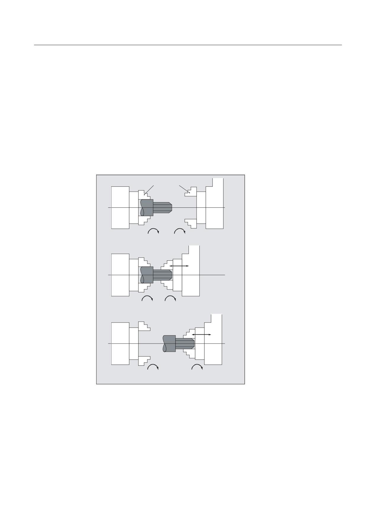
Axis couplings

9.5 Synchronous spindle

9.5.1

Synchronous spindle: Programming (COUPDEF, COUPDEL, COUPON,

COUPONC, COUPOF, COUPOFS, COUPRES, WAITC)

Function

The synchronous spindle function facilitates synchronous traversing of two spindles

(following spindle FS and leading spindle LS), e.g. for workpiece transfer on-the-fly.

The function supports the following modes:

● Speed synchronism (nFS = n LS)

● position synchronism (ϕFS = ϕLS)

● position synchronism with angular offset (ϕFS = ϕLS+ ∆ϕ)

&KXFNV

6SLQGOH

Job Planning

Programming Manual, 03/2010, 6FC5398-2BP20-1BA0

535

Axis couplings

9.5 Synchronous spindle

Multi-edge machining can even be supported by means of the specification of a

transformation ratio not equal to 1 between the leading and following spindles.

Syntax

COUPDEF(<FS>,<LS>,<TFS>,<TLS>,<block change>,<coupling type>)

COUPON(<FS>,<LS>,<POSFS>)

COUPONC(<FS>,<LS>)

COUPOF(<FS>,<LS>,<POSFS>,<POSLS>)

COUPOFS(<FS>,<LS>)

COUPOFS(<FS>,<LS>,<POSFS>)

COUPRES(<FS>,<LS>)

COUPDEL(<FS>,<LS>)

WAITC(<FS>,<block change>,<LS>,<block change>)

Note

Abbreviated notation

The COUPOF, COUPOFS, COUPRES, and COUPDEL statements support abbreviated notation without

specification of the leading spindle.

Meaning

COUPDEF:

Define/change coupling on user-specific basis

COUPON:

Activate coupling. The following spindle synchronizes to the leading

spindle based on the actual speed

COUPONC:

Coupling when activating with previous programming of M3 S... or

M4 S

A difference in speed for the following spindle is transferred

immediately.

COUPOF:

Deactivate coupling.

• With immediate block change:

COUPOF(<S2>,<S1>)

• Block change only after <POSFS> or <POSLS> deactivation

position(s) has (have) been crossed:

COUPOF(<S2>,<S1>,<POSFS>)

COUPOF(<S2>,<S1>,<POSFS>,<POSLS>)

Job Planning

536

Programming Manual, 03/2010, 6FC5398-2BP20-1BA0

Axis couplings

9.5 Synchronous spindle

COUPOFS:

Deactivating a coupling with stop of following spindle.

Block change as quickly as possible with immediate block change:

COUPOFS(<S2>,<S1>)

Block change only after passing the switch-off position:

COUPOFS(<S2>,<S1>,<POSFS>)

COUPRES:

Reset coupling parameters to configured MD and SD

COUPDEL:

Delete user-defined coupling

WAITC:

Wait for synchronized run condition

(NOC are increased to IPO during block changes)

<FS>:

Designation of following spindle

Optional parameters:

<LS>:

Designation of main spindle

Specification with spindle number: e.g. S2, S1

<TFS>, <TLS>:

Transformation ratio between FS and LS.

<TFS> = numerator, <TLS> = denominator

Default: <TFS> / <TLS> = 1.0 ; specification of denominator optional

Block change behavior

The block change is:

"NOC"

Immediately

"FINE"

On reaching "Synchronism fine"

"COARSE"

On reaching "Synchronism coarse"

"IPOSTOP"

On reaching IPOSTOP; in other words, after

setpoint-based synchronism (default)

The block change behavior is effective modally.

Coupling type: Coupling between FS and LS

"DV"

Setpoint linkage (default)

"AV"

Actual value coupling

"VV"

Speed coupling

The coupling type is modal.

<POSFS>:

Angle offset between leading and following spindles

Range of values:

0°… 359.999°

Switch-off positions of the following and leading spindles

"The block change is enabled once POSFS, POSLS has been

passed"

Range of values:

0°… 359.999°

Job Planning

Programming Manual, 03/2010, 6FC5398-2BP20-1BA0

537

Axis couplings

9.5 Synchronous spindle

Examples

Example 1: Machining with leading and following spindles

Programming

Comment

; Leading spindle = master spindle = spindle 1

; Following spindle = spindle 2

N05 M3 S3000 M2=4 S2=500

; Leading spindle rotates at 3000 rpm,

following spindle at 500 rpm.

N10 COUPDEF(S2,S1,1,1,"NOC","Dv")

; Definition of the coupling (can also be configured).

N70 SPCON

; Bring leading spindle into closed-loop position control

(setpoint coupling).

N75 SPCON(2)

; Bring following spindle into closed-loop position control.

N80 COUPON(S2,S1,45)

; On-the-fly coupling to offset position = 45 degrees.

N200 FA[S2]=100

; Positioning speed = 100 degrees/min

N205 SPOS[2]=IC(-90)

; Traverse with 90 degree overlay in negative direction.

N210 WAITC(S2,"Fine")

; Wait for "fine" synchronism.

N212 G1 X... Y... F...

; Machining

N215 SPOS[2]=IC(180)

; Traverse with 180 degree overlay in the positive

direction.

N220 G4 S50

; Dwell time = 50 revolutions of the master spindle

N225 FA[S2]=0

; Activate configured velocity (MD).

N230 SPOS[2]=IC(-7200)

;

20 revolutions. Move with configured velocity in the

negative direction.

N350 COUPOF(S2,S1)

; Couple-out on-the-fly, S=S2=3000

N355 SPOSA[2]=0

; Stop FS at zero degrees.

N360 G0 X0 Y0

N365 WAITS(2)

; Wait for spindle 2.

N370 M5

; Stop FS.

N375 M30

Job Planning

538

Programming Manual, 03/2010, 6FC5398-2BP20-1BA0

Axis couplings

9.5 Synchronous spindle

Example 2: Programming a difference in speed

Programming

Comment

; Leading spindle = master spindle = spindle 1

; Following spindle = spindle 2

N01 M3 S500

; Leading spindle rotates at 500 rpm.

N02 M2=3 S2=300

; Following spindle rotates at 300 rpm.

N10 G4 F1

; Dwell time of master spindle.

N15 COUPDEF (S2,S1,-1)

; Coupling factor with ratio -1:1

N20 COUPON (S2,S1)

; Activate coupling. The speed of the following spindle results from

the speed of the leading spindle and coupling factor.

N26 M2=3 S2=100

; Programming a difference in speed.

Example 3: Examples of transfer of a movement for difference in speed

1. Activate coupling during previous programming of following spindle with COUPON

Programming

Comment

; Leading spindle = master spindle = spindle 1

; Following spindle = spindle 2

N05 M3 S100 M2=3 S2=200

; Leading spindle rotates at 100 rpm, following spindle at 200 rpm.

N10 G4 F5

; Dwell time = 5 seconds of master spindle

N15 COUPDEF(S2,S1,1)

; Transformation ratio of FS to LS is 1.0 (default).

N20 COUPON(S2,S1)

; On-the-fly coupling to the leading spindle.

N10 G4 F5

; Following spindle rotates at 100 rpm.

2. Activate coupling during previous programming of following spindle with COUPONC

Programming

Comment

; Leading spindle = master spindle = spindle 1

; Following spindle = spindle 2

N05 M3 S100 M2=3 S2=200

; Leading spindle rotates at 100 rpm, following spindle at 200 rpm.

N10 G4 F5

; Dwell time = 5 seconds of master spindle

N15 COUPDEF(S2,S1,1)

; Transformation ratio of FS to LS is 1.0 (default).

N20 COUPONC(S2,S1)

; On-the-fly coupling to leading spindle and transfer previous speed

to S2.

N10 G4 F5

; S2 rotates at 100 rpm + 200 rpm = 300 rpm

Job Planning

Programming Manual, 03/2010, 6FC5398-2BP20-1BA0

539

Axis couplings

9.5 Synchronous spindle

3. Activate coupling with following spindle stationary with COUPON

Programming

Comment

; Leading spindle = master spindle = spindle 1

; Following spindle = spindle 2

N05 SPOS=10 SPOS[2]=20

; Following spindle S2 in positioning mode.

N15 COUPDEF(S2,S1,1)

; Transformation ratio of FS to LS is 1.0 (default).

N20 COUPON(S2,S1)

; On-the-fly coupling to the leading spindle.

N10 G4 F1

; Coupling is closed, S2 stops at 20 degrees.

4. Activate coupling with following spindle stationary with COUPONC

Note

Positioning or axis mode

If the following spindle is in positioning or axis mode before coupling, then the following

spindle behaves the same for COUPON(<FS>,<LS>) and COUPONC(<FS>,<LS>).

NOTICE

Leading spindle and axis operation

If, prior to the coupling being defined, the leading spindle is in axis operation, the velocity

limit value from machine data

MD32000 $MA_MAX_AX_VELO (maximum axis velocity) will still apply even after the

coupling is activated.

To avoid this behavior, the axis must be switched to spindle mode (M3 S... or M4 S...) prior

to the coupling being defined.

Further information

Define synchronized spindle pair

Configured coupling:

For the configured coupling, the leading and following spindles are defined in machine data.

The configured spindles cannot be changed in the part program. The coupling can be

parameterized in the part program using COUPDEF (on condition that no write protection is

valid).

User-defined coupling:

COUPDEF can be used to redefine or change a coupling in the part program. If a coupling is

already active, it has to be deleted first with COUPDEL before a new coupling is defined.

Define coupling: COUPDEF

A coupling is defined in its entirety by:

COUPDEF(<FS>,<LS>,<TFS>,<TLS>, block change behavior, coupling type)

Job Planning

540

Programming Manual, 03/2010, 6FC5398-2BP20-1BA0

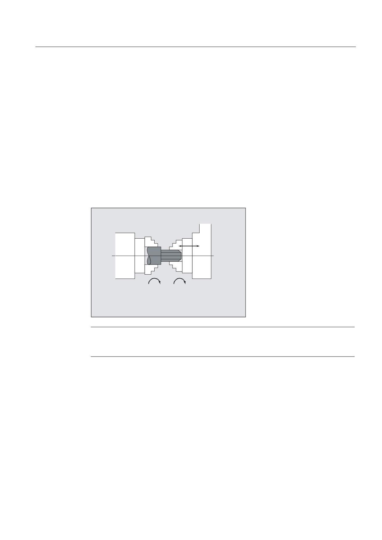
Axis couplings

9.5 Synchronous spindle

Following spindle (FS) and leading spindle (LS)

The coupling is uniquely defined using the axis names for the following spindle (FS) and the

leading spindle (LS). The axis names have to be programmed with every COUPDEF operation.

The other coupling parameters are modal and only have to be programmed if they change.

Example:

COUPDEF(S2,S1)

Transformation ratio, TFS / TLS

The transformation ratio is specified as a speed ratio between the following spindle

(numerator) and the leading spindle (denominator). The numerator must be programmed. In

the absence of a programmed value, the denominator is set to = 1.0.

Example:

Following spindle S2 and leading spindle S1, transformation ratio = 1 / 4 = 0.25.

COUPDEF(S2,S1,1.0, 4.0)

6SLQGOH

/HDG

)ROORZLQJ

VSLQGOH

Note

The transformation ratio can also be changed on-the-fly (when the coupling is active and the

spindles are rotating).

Block change behavior NOC, FINE, COARSE, IPOSTOP

The following abbreviated notation can be used when programming the block change

behavior:

● "NO": Immediately (default)

● "FI": On reaching "Synchronism fine"

● "CO": On reaching "Synchronism coarse"

● "IP": On reaching IPOSTOP; in other words, after setpoint-based synchronism

Job Planning

Programming Manual, 03/2010, 6FC5398-2BP20-1BA0

541

Axis couplings

9.5 Synchronous spindle

Type of coupling DV, AV

CAUTION

The coupling type may be changed only when the coupling is deactivated!

Activate synchronized mode COUPON, POSFS

● Activation of coupling with any angle reference between LS and FS:

- COUPON(S2,S1)

- COUPON(S2,S1,<POSFS>)

- COUPON(S2)

● Activation of coupling with angular offset <POSFS>

Position-synchronized coupling for profiled workpieces.

<POSFS>refers to the 0° position of the lead spindle in the positive direction of rotation

<POSFS> value range: 0°… 359.999°

- COUPON(S2,S1,30)

You can use this method to change the angle offset even when the coupling is already

active.

Position the following spindle

When the synchronized spindle coupling is active, following spindles can also be positioned

within the ±180° range independently of the motion initiated by the master spindle.

Positioning SPOS

The following spindle can be interpolated with SPOS=….

Example:

SPOS[2]=IC(-90)

Further information about SPOS appears in:

Reference:

Programming Manual, Basics

Difference in speed M3 S... or M4 S...

A difference in speed results from signed superimposition of two sources of speed and is

programmed again for the following spindle e.g. with S<n>=... or M<n>=3, M<n>=4 in the speed

control mode during an active synchronized spindle coupling. During the process, this speed

component is derived from the main spindle using the coupling factor and the following

spindle added to this with the correct prefix.

Note

When the direction of rotation is M3 or M4, the speed S... also has to be reprogrammed

because otherwise an alarm is triggered to report missing programming.

For more information about the speed difference, please refer to:

Reference:

Function Manual, Extended Functions; Synchronous Spindle (S3).

Job Planning

542

Programming Manual, 03/2010, 6FC5398-2BP20-1BA0

Axis couplings

9.5 Synchronous spindle

Difference in speed for COUPONC

Transfer of a movement for difference in speed

When a synchronous spindle coupling is activated with COUPONC a currently active speed is

overlaid on the following spindle (M3 S... or M4 S...).

Note

Enabling overlaying

Overlay of a spindle speed ( M3 S... or M4 S...) using a synchronous spindle coupling

COUPONC only becomes effective if the overlay has been enabled.

Dynamic restriction of the leading spindle

The dynamic responses of the leading spindle have to be restricted to such an extent that

when overlaying is applied to the following spindle, its dynamics limit values are not

exceeded.

Velocity, acceleration: FA, ACC, OVRA, VELOLIMA

Axial velocity and acceleration of a following spindle can be programmed with:

● FA[SPI(S<n>)] or FA[S<n>] (axial velocity)

● ACC[SPI(S<n>)] or ACC[S<n>] (axial acceleration)

● OVRA[SPI(S<n>)] and OVRA[S<n>] (axial override)

● VELOLIMA[SPI(S<n>)] and VELOLIMA[S<n>] (increase and reduction of axial velocity

respectively)

When <n> = 1, 2, 3, ... (spindle numbers of the following spindles)

Reference:

Programming Manual Fundamentals

Note

Acceleration component JERKLIMA[S<n>]

Programming an increase or reduction in axial velocity is currently ineffective for spindles.

Further information about configuring the axial dynamic response is provided in:

Reference:

Function Manual Extended Functions; Rotary Axes (R2)

Programmable block change behavior WAITC

WAITC can be used to define block change behavior, for example after a change to coupling

parameters or positioning actions, with a variety of synchronism conditions (coarse, fine,

IPOSTOP). If no synchronism conditions are specified, the block change behavior specified in

the COUPDEF definition will apply.

Example:

Wait for synchronism condition according to COUPDEF to be fulfilled

WAITC( )

Wait for synchronism condition FINE to be fulfilled for following spindle S2 and COARSE to be

fulfilled for following spindle S4:

WAITC(S2,"FINE",S4,"COARSE")

Job Planning

Programming Manual, 03/2010, 6FC5398-2BP20-1BA0

543

SINUMERIK 840D sl/828D. Job Planning. Programming Manual (2010-2018) - page 21