SINUMERIK 840D sl/828D. Job Planning. Programming Manual (2010-2018) - page 9

Axis couplings
13.2 Curve tables (CTAB)
<following axis>:
Axis whose motion is to be calculated using the curve table (optional)
<leasing axis>:
Axis providing the master values for the calculation of the following axis
motion (optional)
<following value>:
Following axis value for reading the associated leading axis value for
CTABINV
<leading value>:
Leading axis value:
● For reading the associated following axis value with CTAB
or
● For the selection of the curve segment with CTABSSV/CTABSEV
<approximate
The assignment of a leading axis value to a following axis value with
value>:
CTABINV must not always be unique. CTABINV requires, therefore, an ap-
proximate value for the expected leading axis value as a parameter.
<a>:
Lower limit of the master value interval with CTABTMIN/CTABTMAX
<b>:
Upper limit of the master value interval with CTABTMIN/CTABTMAX
Note:
The master value interval <a> to <b> always has to be within the curve
table's definition range.
Examples
Example 1:
Define following axis and leading axis values at the start and end of the curve table, along with
the minimum and maximum values of the following axis in the entire definition range of the
curve table.
Program code
Comment
N10 DEF REAL STARTPOS
N20 DEF REAL ENDPOS
N30 DEF REAL STARTPARA
N40 DEF REAL ENDPARA
N50 DEF REAL MINVAL
N60 DEF REAL MAXVAL
N70 DEF REAL GRADIENT
N100 CTABDEF(Y,X,1,0)
; Start of table definition
N110 X0 Y10
; Start position 1st table segment
N120 X30 Y40
; End position 1st table segment =
start position 2nd table segment
N130 X60 Y5
; End position 2nd table segment = ...
N140 X70 Y30
N150 X80 Y20
N160 CTABEND
; End of table definition.
N200 STARTPOS=CTABTSV(1,GRADIENT)
; Following axis value at start of curve table
= 10
N210 ENDPOS=CTABTEV(1,GRADIENT)
; Following axis value at end of curve table
= 20
Job Planning
558
Programming Manual, 12/2018, A5E40869460B AB
Axis couplings
13.2 Curve tables (CTAB)
Program code
Comment
N220 STARTPARA=CTABTSP(1,GRADIENT)
; Master axis value at start of curve table =
0
N230 ENDPARA=CTABTEP(1,GRADIENT)
; Master axis value at end of curve table = 80
N240 MINVAL=CTABTMIN(1)
; Minimum value of following axis with Y=5
N250 MAXVAL=CTABTMAX(1)
; Maximum value of following axis with Y=40
Example 2:
Determination of following axis values at the start and end of the curve segment associated
with leading axis value X=30.
Program code
Comment
N10 DEF REAL STARTPOS
N20 DEF REAL ENDPOS
N30 DEF REAL GRADIENT
N100 CTABDEF(Y,X,1,0)
; Start of table definition.
N110 X0 Y0
; Start position 1st table segment
N120 X20 Y10
; End position 1st table segment =
start position 2nd table segment
N130 X40 Y40
; End position 2nd table segment = ...
N140 X60 Y10
N150 X80 Y0
N160 CTABEND
; End of table definition.
N200 STARTPOS=CTABSSV(30.0,1,GRADIENT)
; Start position Y in 2nd segment = 10
N210 ENDPOS=CTABSEV(30.0,1,GRADIENT)
; End position Y in 2nd segment = 40
Further information
Use in synchronized actions
All commands for reading curve table values can also be used in synchronized actions (see
also the chapter titled "Motion-synchronous actions").
When using the CTABINV, CTABTMIN, and CTABTMAX commands, make sure that:
● Sufficient NC power is available at the time of execution
or
● The number of segments in the curve table is queried prior to the call, so that the table
concerned can be subdivided if necessary
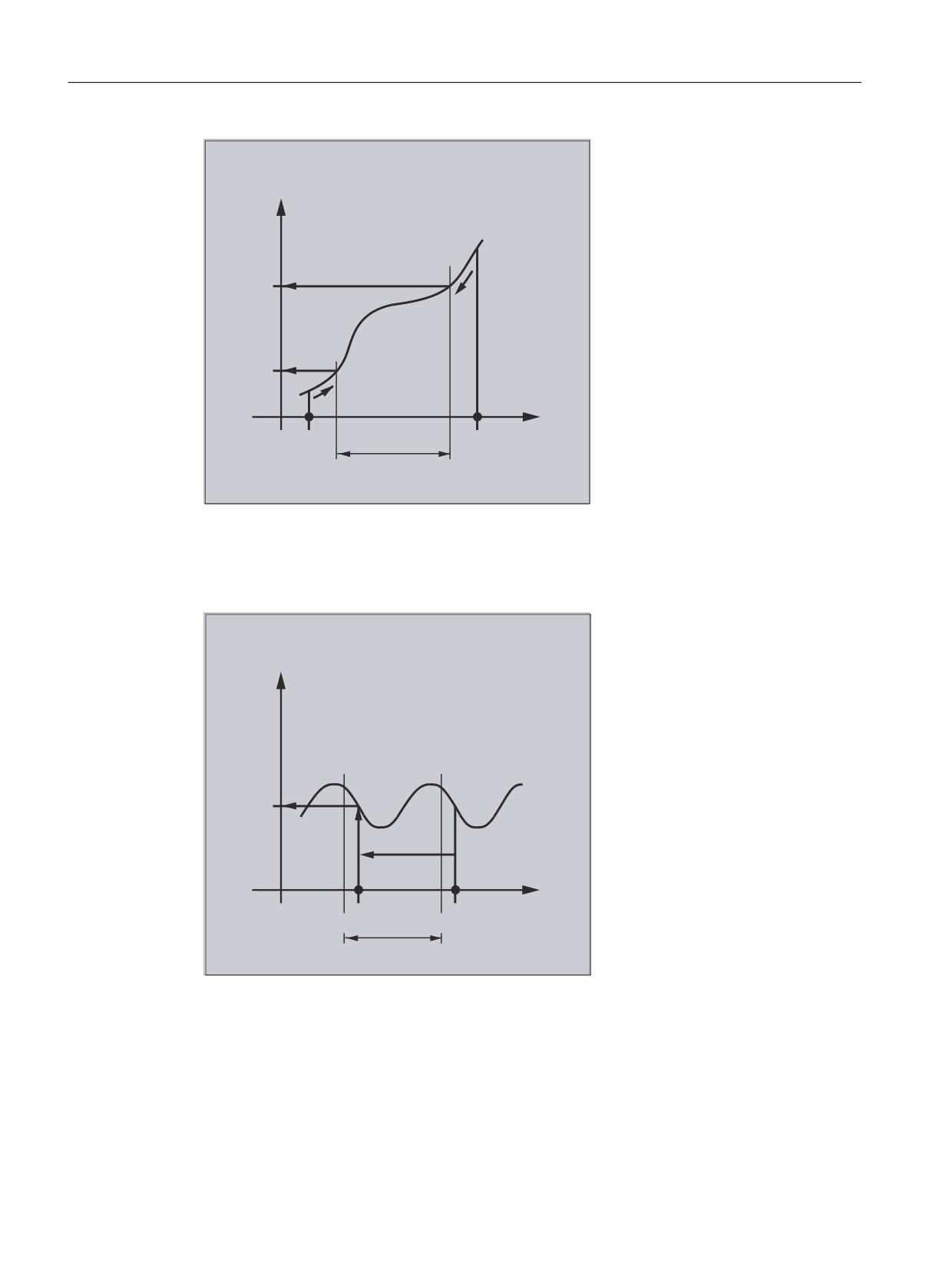
CTAB with non-periodic curve tables
If the specified <master value> is outside the definition range, the upper or lower limit will
be output as the following value:
Job Planning
Programming Manual, 12/2018, A5E40869460B AB
559
Axis couplings
13.2 Curve tables (CTAB)
6ODYH YDOXH
)
)
0DVWHU
/
'HILQLWLRQ UDQJH
/
YDOXH
CTAB with periodic curve tables
If the specified <master value> is outside the definition range, the master value is evaluated
modulo of the definition range and the corresponding following value is output:
6ODYH YDOXH
)
0DVWHU
/
'HILQLWLRQ UDQJH
YDOXH
Approximate value for CTABINV
The CTABINV command, therefore, requires an approximate value for the expected master
value. CTABINV returns the leading value that is closest to the approximate value. The
approximate value can be, for example, the master value from the previous interpolator clock
cycle.
Job Planning
560
Programming Manual, 12/2018, A5E40869460B AB
Axis couplings
13.2 Curve tables (CTAB)
Incline of the curve table function
The output of the incline (<gradient>) makes it possible to calculate the velocity of the
leading or following axis at the corresponding position.
Specification of the leading or following axis
The optional specification of the leading and/or following axis is important if the leading and
following axes are configured in different length units.
CTABSSV, CTABSEV
The CTABSSV and CTABSEV commands are not suitable to query programmed segments in
the following cases:
● Circles or involutes are programmed.
● Chamfer or rounding with CHF/ RND is active
● Smoothing with G643 is active
● NC block compression with COMPON/COMPCURV/COMPCAD is active
13.2.7
Curve tables: Check use of resources (CTABNO, CTABNOMEM, CTABFNO,
CTABSEGID, CTABSEG, CTABFSEG, CTABMSEG, CTABPOLID, CTABPOL,
CTABFPOL, CTABMPOL)
The programmer can use these commands to obtain up-to-date information about the use of
resources for curve tables, table segments, and polynomials.
Syntax
CTABNO
CTABNOMEM(<memory location>)
CTABFNO(<memory location>)
CTABSEGID(<n>,<memory location>)
CTABSEG(<memory location>,<segment type>)
CTABFSEG(<memory location>,<segment type>)
CTABMSEG(<memory location>,<segment type>)
CTABPOLID(<n>)
CTABPOL(<memory location>)
CTABFPOL(<memory location>)
CTABMPOL(<memory location>)
Meaning
CTABNO:
Determine the total number of defined curve tables (in the static and the dy-
namic NC memory)
CTABNOMEM:
Determine the number of defined curve tables in the specified <memory
location>
CTABFNO:
Determine the number of curve tables remaining possible in the specified
<memory location>
Job Planning
Programming Manual, 12/2018, A5E40869460B AB
561

Axis couplings
13.2 Curve tables (CTAB)
CTABSEGID:
Determine the number of curve segments of the specified <segment
type> used by curve table number <n>
CTABSEG:
Determine the number of curve segments of the specified <segment
type> used in the specified <memory location>
CTABFSEG:
Determine the number of curve segments of the specified <segment
type> remaining possible in the specified <memory location>
CTABMSEG:
Determine the maximum possible number of curve segments of the specified
<segment type> in the specified <memory location>
CTABPOLID:
Determine the number of curve polynomials used by curve table number <n>
CTABPOL:
Determine the number of curve polynomials used in the specified <memory
location>
CTABFPOL:
Determine the number of curve polynomials remaining possible in the speci-
fied <memory location>
CTABMPOL:
Determine the maximum possible number of curve polynomials in the speci-
fied <memory location>
<n>:
Number (ID) of curve table
<memory
Specification of memory location (optional)
location>:
"SRAM"
Static NC memory
"DRAM"
Dynamic NC memory
Note:
If a value is not programmed for this parameter, the default memory location
set with MD20905 $MC_CTAB_DEFAULT_MEMORY_TYPE is used.
<segment type>:
Specification of segment type (optional)
"L"
Linear segments
"P"
Polynomial segments
Note:
If no value is programmed for this parameter, the sum of the linear and poly-
nomial segments is output.
Job Planning
562
Programming Manual, 12/2018, A5E40869460B AB
Axis couplings
13.3 Axial master value coupling (LEADON, LEADOF)
13.3
Axial master value coupling (LEADON, LEADOF)
Note
This function is not available for SINUMERIK 828D!
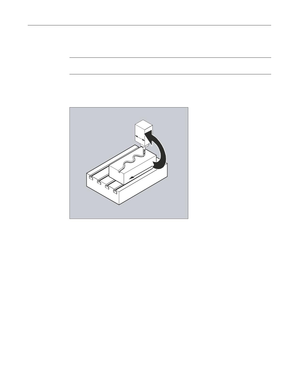
With the axial master value coupling, a leading and a following axis are moved in synchronism.
It is possible to assign the position of the following axis via a curve table or the resulting
polynomial uniquely to a position of the leading axis - simulated if necessary.
<
;
The leading axis is the axis which supplies the input values for the curve table. The following
axis is the axis, which takes the positions calculated by means of the curve table.
Actual value and setpoint coupling
The following can be used as the master value, i.e. as the output values for position calculation
of the following axis:
● Actual values of the leading axis position: Actual value coupling
● Setpoints of the leading axis position: Setpoint value coupling
The master value coupling always applies in the basic coordinate system.
For information on the creation of curve tables, see Section "Curve tables".
Syntax
LEADON(<following axis>,<leading axis>,<n>)
LEADOF(<following axis>,<leading axis>)
or deactivation without specifying the leading axis:
LEADOF(<following axis>)
Job Planning
Programming Manual, 12/2018, A5E40869460B AB
563

Axis couplings
13.3 Axial master value coupling (LEADON, LEADOF)
The master value coupling can be activated/deactivated both from the part program and also
during motion from synchronized actions.
Meaning
LEADON:
Activate master value coupling
LEADOF:
Deactivate master value coupling
<following axis>:
Following axis
<leasing axis>:
Leading axis
<n>:
Curve table number
$SA_LEAD_TYPE:
Switching between setpoint and actual value coupling
Deactivate master value coupling, LEADOF
When you deactivate the master value coupling, the following axis becomes a normal
command axis again!
Axial master value coupling and different operating states, RESET
Depending on the setting in the machine data, the master value couplings are deactivated with
RESET.
Example of master value coupling from synchronous action
In a pressing plant, an ordinary mechanical coupling between a leading axis (stanchion shaft)
and axis of a transfer system comprising transfer axes and auxiliary axes is to be replaced by
an electronic coupling system.
It demonstrates how a mechanical transfer system is replaced by an electronic transfer system.
The coupling and decoupling processes are implemented as static synchronized actions.
From the leading axis LV (stanchion shaft), transfer axes and auxiliary axes are controlled as
following axes that are defined via curve tables.
Following axes
X feed or longitudinal axis
YL closing or transverse axis
ZL lifting axis
U roll feed, auxiliary axis
V guide head, auxiliary axis
W greasing, auxiliary axis
Actions
The actions that occur include, for example, the following synchronized actions:
● Activate coupling, LEADON(<following axis>,<leading axis>,<curve table
number>)
● Deactivate coupling, LEADOF(<following axis>,<leading axis>)
● Set actual value, PRESETON(<axis>,<value>)
● Set marker, $AC_MARKER[i]=<value>
Job Planning
564
Programming Manual, 12/2018, A5E40869460B AB
Axis couplings
13.3 Axial master value coupling (LEADON, LEADOF)
● Coupling type: real/virtual master value
● Approaching axis positions, POS[<axis>]=<value>
Conditions
Fast digital inputs, real-time variables $AC_MARKER and position comparisons are linked using
the Boolean operator AND for evaluation as conditions.
Note
In the following example, line change, indentation and bold type are used for the sole purpose
of improving readability of the program. For the control, everything that follows a line number
constitutes a single line.
Comment
Program code
Comment
; Defines all static synchronized actions.
; ****Reset marker
N2 $AC_MARKER[0]=0 $AC_MARKER[1]=0 $AC_MARKER[2]=0 $AC_MARKER[3]=0 $AC_MARKER[4]=0 $AC_MARKER[5]=0
$AC_MARKER[6]=0 $AC_MARKER[7]=0
; **** E1 0=>1 transfer ON
N10 IDS=1 EVERY ($A_IN[1]==1) AND ($A_IN[16]==1) AND ($AC_MARKER[0]==0)
DO LEADON(X,LW,1) LEADON(YL,LW,2) LEADON(ZL,LW,3) $AC_MARKER[0]=1
;**** E1 0=>1 coupling roller feed ON
N20 IDS=11 EVERY ($A_IN[1]==1) AND ($A_IN[5]==0) AND ($AC_MARKER[5]==0)
DO LEADON(U,LW,4) PRESETON(U,0) $AC_MARKER[5]=1
; **** E1 0->1 coupling alignment head ON
N21 IDS=12 EVERY ($A_IN[1]==1) AND ($A_IN[5]==0) AND ($AC_MARKER[6]==0)
DO LEADON(V,LW,4) PRESETON(V,0) $AC_MARKER[6]=1
; **** E1 0->1 lubrication coupling ON
N22 IDS=13 EVERY ($A_IN[1]==1) AND ($A_IN[5]==0) AND ($AC_MARKER[7]==0)
DO LEADON(W,LW,4) PRESETON(W,0) $AC_MARKER[7]=1
; **** E2 0=>1 coupling OFF
N30 IDS=3 EVERY ($A_IN[2]==1)
DO LEADOF(X,LW) LEADOF(YL,LW) LEADOF(ZL,LW) LEADOF(U,LW) LEADOF(V,LW) LEADOF(W,LW) $AC_MARKER[0]=0
$AC_MARKER[1]=0 $AC_MARKER[3]=0 $AC_MARKER[4]=0 $AC_MARKER[5]=0 $AC_MARKER[6]=0 $AC_MARKER[7]=0
N110 G04 F01
N120 M30
Description
Master value coupling requires synchronization of the leading and the following axes. This
synchronization can only be achieved if the following axis is inside the tolerance range of the
curve definition calculated from the curve table when the master value coupling is activated.
The tolerance range for the position of the following axis is defined via machine data MD
37200: COUPLE_POS_POL_COARSE A_LEAD_TYPE.
Job Planning
Programming Manual, 12/2018, A5E40869460B AB
565
Axis couplings
13.3 Axial master value coupling (LEADON, LEADOF)
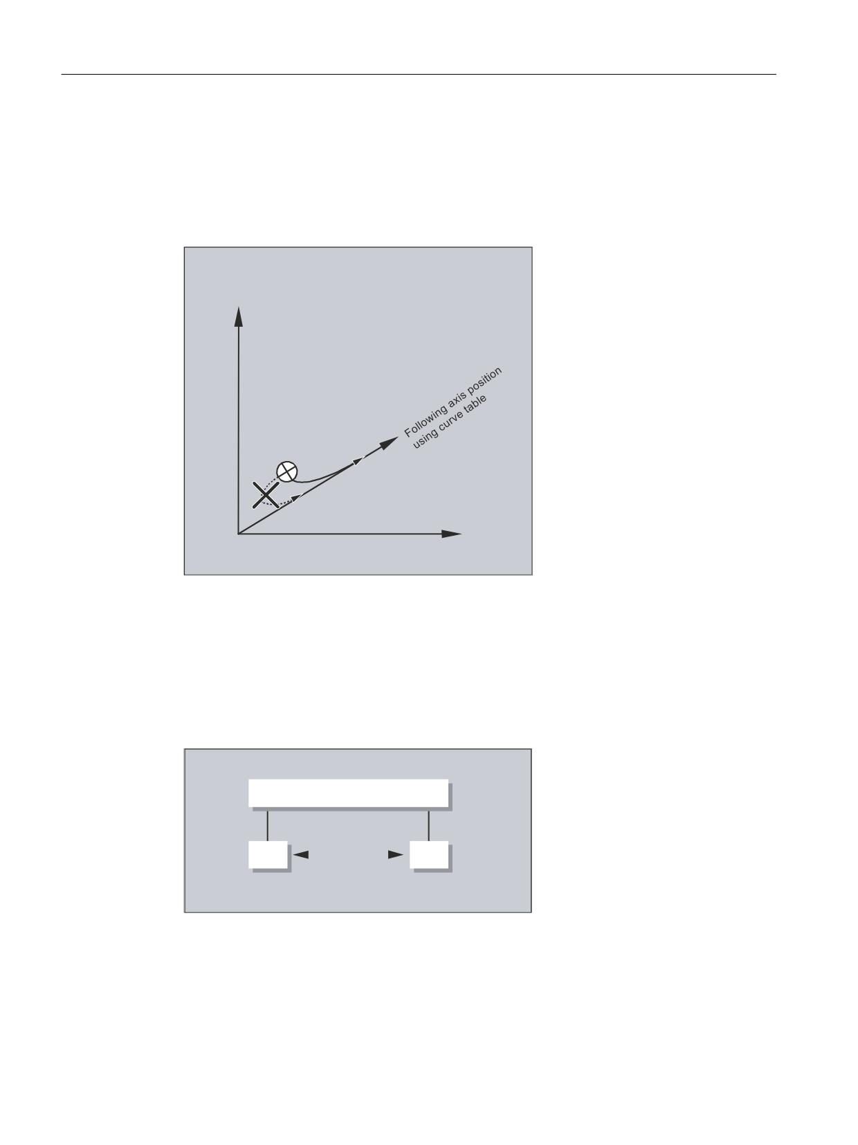
If the following axis is not yet at the correct position when the master value coupling is activated,
the synchronization run is automatically initiated as soon as the position setpoint value
calculated for the following axis is approximately the real following axis position. During the
synchronization procedure the following axis is traversed in the direction that is defined by the
setpoint speed of the following axis (calculated from master spindle and using the CTAB curve
table).
<
)ROORZLQJ D[LV SRVLWLRQ
<
No synchronism
If the following axis position calculated moves away from the current following axis position
when the master value coupling is activated, it is not possible to establish synchronization.
Actual value and setpoint coupling
Setpoint coupling provides better synchronization of the leading and following axis than actual
value coupling and is therefore set by default.
1&8
6HWSRLQW YDOXH FRXSOLQJ
$[
$[
$FWXDO YDOXH FRXSOLQJ
Setpoint coupling is only possible if the leading and following axis are interpolated by the same
NCU. With an external leading axis, the following axis can only be coupled to the leading axis
via the actual values.
Job Planning
566
Programming Manual, 12/2018, A5E40869460B AB
Axis couplings
13.3 Axial master value coupling (LEADON, LEADOF)
1&8
1&8
$[
$[
$FWXDO YDOXH FRXSOLQJ
A switchover can be programmed via setting data $SA_LEAD_TYPE.
You must always switch between the actual-value and setpoint coupling when the following
axis stops. It is only possible to resynchronize after switchover when the axis is motionless.
Application example
You cannot read the actual values without error during large machine vibrations. If you use
master value coupling in press transfer, it might be necessary to switchover from actual-value
coupling to setpoint coupling in the work steps with the greatest vibrations.
Master value simulation with setpoint coupling
Via machine data, you can disconnect the interpolator for the leading axis from the servo. In
this way you can generate setpoints for setpoint coupling without actually moving the leading
axis.
Master values generated from a setpoint link can be read from the following variables so that
they can be used, for example, in synchronized actions:
- $AA_LEAD_P
Master value position
- $AA_LEAD_V
Master value velocity
Create master value
As an option, master values can be generated with other self-programmed methods. The
master values generated in this way are written to and read from variables
- $AA_LEAD_SP
Master value position
- $AA_LEAD_SV
Master value velocity
Before you use these variables, the setting data $SA_LEAD_TYPE = 2 must be set.
Status of coupling
You can query the status of the coupling in the NC program with the following system variable:
$AA_COUP_ACT[[axis]]
0: No coupling active
16: Master value coupling active
Status management for synchronized actions
Switching and coupling events are managed via real-time variables:
$AC_MARKER[i] = n
managed with:
Job Planning
Programming Manual, 12/2018, A5E40869460B AB
567
Axis couplings
13.3 Axial master value coupling (LEADON, LEADOF)
i flag number
n status value
Job Planning
568
Programming Manual, 12/2018, A5E40869460B AB
Axis couplings
13.4 Electronic gear (EG)
13.4
Electronic gear (EG)
The "Electronic gear" function allows you to control the movement of a following axis according
to linear traversing block as a function of up to five leading axes. The relationship between
each leading axis and the following axis is defined by the coupling factor.
The following axis motion part is calculated by an addition of the individual leading axis motion
parts multiplied by their respective coupling factors. When an EG axis grouping is activated,
it is possible to synchronize the following axes in relation to a defined position. A gear group
can be:
● Defined
● Activated
● Deactivated
● Deleted
The following axis movement can be optionally derived from
● Setpoints of the leading axes, as well as
● Actual values of leading axes.
Non-linear relationships between each leading axis and the following axis can also be realized
as extension using curve tables (see "Path traversing behavior" section). Electronic gears can
be cascaded, i.e., the following axis of an electronic gear can be the leading axis for a further
electronic gear.
13.4.1
Defining an electronic gear (EGDEF)
An EG axis group is defined by specifying the following axis and at least one, however not
more than five, leading axis, each with the relevant coupling type.
Requirement
Requirements for defining an EG axis group:
It is not permissible to define an axis coupling for the following axis (or an existing one must
first be deleted with EGDEL).
Syntax
EGDEF(following axis,leading axis1,coupling type1,leading
axis2,coupling type2,...)
Meaning
EGDEF:
Definition of an electronic gear
Following axis:
Axis that is influenced by the leading axes
Job Planning
Programming Manual, 12/2018, A5E40869460B AB
569
Axis couplings
13.4 Electronic gear (EG)
Leading axis1
Axes that influence the following axis
,...,
Leading axis5
Coupling type1
Coupling type
,...,
The coupling type does not need to be the same for all leading axes and
Coupling type5
must be programmed separately for each individual master.
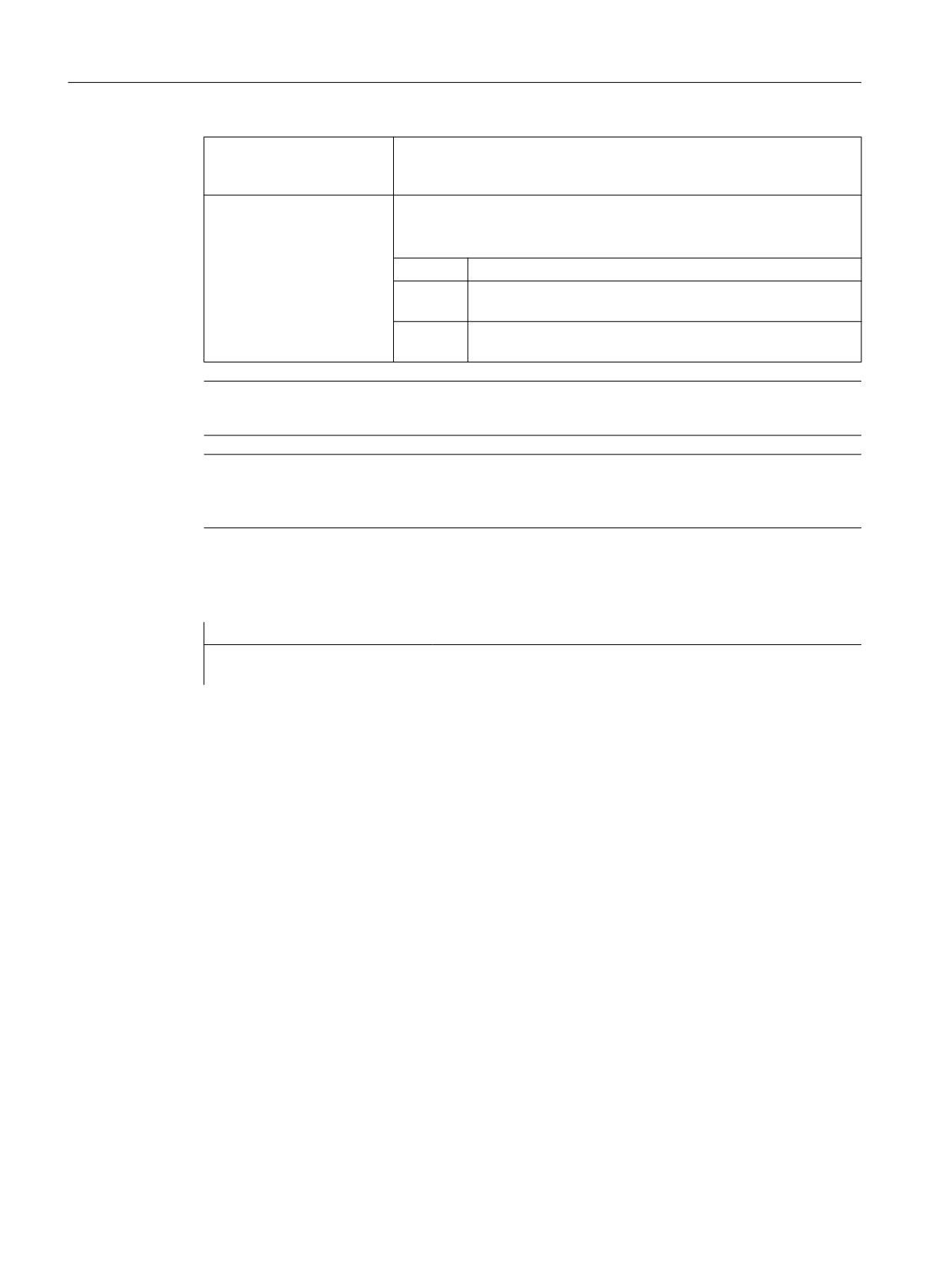
Value:
Meaning:
0
The following axis is influenced by the actual value of the
corresponding leading axis.
1
The following axis is influenced by the setpoint of the corre-
sponding leading axis.
Note
The coupling factors are preset to zero when the EG axis grouping is defined.
Note
EGDEF triggers preprocessing stop. The gearbox definition with EGDEF should also be used
unaltered if, for systems, one or more leading axes affect the following axis via a curve table.
Example
Program code
Comment
EGDEF(C,B,1,Z,1,Y,1)
; Definition of an EG axis group. Leading axes B, Z, Y
influence the following axis C via the setpoint.
13.4.2
Switch-in the electronic gearbox (EGON, EGONSYN, EGONSYNE)
There are 3 ways to switch-in an EG axis group.
Syntax
Variant 1:
The EG axis group is selectively switched-in without synchronization with:
EGON(FA,"block change mode",LA1,Z1,N1,LA2,Z2,N2,...,LA5,Z5,N5)
Variant 2:
The EG axis group is selectively activated with synchronization with:
EGONSYN(FA,"block change mode",SynPosFA,[,LAi,SynPosLAi,Zi,Ni])
Variant 3:
The EG axis group is selectively switched-in with synchronization and the approach mode
specified with:
EGONSYNE(FA,"block change mode",SynPosFA,approach
mode[,LAi,SynPosLAi,Zi,Ni])
Job Planning
570
Programming Manual, 12/2018, A5E40869460B AB

Axis couplings
13.4 Electronic gear (EG)
Meaning
Variant 1:
FA
Following axis
Block change mode:
The following modes can be used:
"NOC"
Block change takes place immediately
"FINE"
Block change is performed in "Fine synchronism"
"COARSE"
Block change is performed in "Coarse synchron-
ism"
"IPOSTOP"
Block change is performed for setpoint-based
synchronism
LA1, ... LA5
Leading axes
Z1, ... Z5
Numerator for coupling factor i
N1, ... N5
Denominator for coupling factor i
Coupling factor i = numerator i/denominator i
Only the leading axes previously specified with the EGDEF command may be programmed in
the activation line. At least one leading axis must be programmed.
Variant 2:
FA
Following axis
Block change mode:
The following modes can be used:
"NOC"
Block change takes place immediately
"FINE"
Block change is performed in "Fine synchron-
ism"
"COARSE"
Block change is performed in "Coarse synchron-
ism"
"IPOSTOP"
Block change is performed for setpoint-based
synchronism
[,LAi,SynPosLAi,Zi,Ni]
(do not write the square brackets)
Min. 1, max. 5 sequences of:
LA1, ... LA5
Leading axes
SynPosLAi
Synchronized position for i-th leading axis
Z1, ... Z5
Numerator for coupling factor i
N1, ... N5
Denominator for coupling factor i
Coupling factor i = numerator i/denominator i
Only leading axes previously specified with the EGDEF command may be programmed in the
activation line. Through the programmed "Synchronized positions" for the following axis
(SynPosFA) and for the leading axes (SynPosLA), positions are defined for which the axis
grouping is interpreted as synchronous. If the electronic gear is not in the synchronized state
when the grouping is switched on, the following axis traverses to its defined synchronized
position.
Job Planning
Programming Manual, 12/2018, A5E40869460B AB
571
Axis couplings
13.4 Electronic gear (EG)
Variant 3:
The parameters correspond to those of variant 2 plus:
Approach mode:
The following modes can be used:
"NTGT"
Approach next tooth gap time-optimized
"NTGP"
Approach next tooth gap path-optimized
"ACN"
Traverse rotary axis in negative direction absolute
"ACP"
Traverse rotary axis in positive direction absolute
"DCT"
Time-optimized for programmed synchronous position
"DCP"
Distance-optimized to the programmed synchronous position
Variant 3 only affects modulo following axes that are coupled to modulo leading axes. Time
optimization takes account of velocity limits of the following axis.
Further information
Description of the switch-in versions
Variant 1:
The positions of the leading axes and following axis at the instant the grouping is switched on
are stored as "Synchronized positions". The "Synchronized positions" can be read with the
system variable $AA_EG_SYN.
Variant 2:
If modulo axes are contained in the coupling group, their position values are modulo-reduced.
This ensures that the next possible synchronized position is approached (so-called relative
synchronization: e.g. the next tooth gap). The synchronized position is only approached if
"Enable following axis override" interface signal DB(30 + axis number), DBX 26 bit 4 is issued
for the following axis. Instead, the program stops at the EGONSYN block and self-clearing
alarm 16771 is output until the above mentioned signal is set.
Variant 3:
The tooth distance (deg.) is calculated like this: 360 * Zi/Ni. If the following axis is stopped at
the time of calling, path optimization returns responds identically to time optimization.
If the following axis is already in motion, NTGP will synchronize at the next tooth gap
irrespective of the current velocity of the following axis. If the following axis is already in motion,
NTGT will synchronize at the next tooth gap depending on the current velocity of the following
axis. The axis is also decelerated, if necessary.
Curve tables
If a curve table is used for one of the leading axes:
Ni
The denominator of the coupling factor for linear coupling must be set to 0. (Denom-
inator 0 would be illegal for linear couplings.) Denominator zero tells the control that
Zi
is the number of the curve table to use. The curve table with the specified number
must already be defined at POWER ON.
LAi
The leading axis specified corresponds to the one specified for coupling via coupling
factor (linear coupling).
Job Planning
572
Programming Manual, 12/2018, A5E40869460B AB
Axis couplings
13.4 Electronic gear (EG)
For more information about using curve tables and cascading and synchronizing electronic
gears, please refer to:
References:
Function Manual Special Functions; Coupled Axes and ESR (M3), "Coupled Motion and
Leading Value Coupling".
Response of the electronic gear for power on, RESET, operating mode change, block search
● No coupling is active after POWER ON.
● The status of active couplings is not affected by RESET or operating mode switchover.
● During block searches, commands for switching, deleting and defining the electronic gear
are not executed or collected, but skipped.
System variables of the electronic gear
By means of the electronic gear's system variables, the part program can determine the current
states of an EG axis grouping and react to them if required.
The system variables of the electronic gearbox are designated as follows:
$AA_EG_ ...
or
$VA_EG_ ...
References:
System Variables Manual
13.4.3
Switching-in the electronic gearbox (EGOFS, EGOFC)
There are 3 different ways to switch-out an active EG axis group.
Programming
Variant 1:
Syntax
Meaning
EGOFS(following axis)
The electronic gear is deactivated. The following axis is braked to a
standstill. This call triggers a preprocessing stop.
Variant 2:
Syntax
Meaning
EGOFS(following axis,leading axis1,
This command parameter setting made it
…,leading axis5)
possible to selectively remove the influence
of the individual leading axes on the following
axis' motion.
At least one leading axis must be specified. The influence of the specified leading axes on the
slave is selectively inhibited. This call triggers a preprocessing stop. If the call still includes
active leading axes, then the slave continues to operate under their influence. If the influence
of all leading axes is excluded by this method, then the following axis is braked to a standstill.
Job Planning
Programming Manual, 12/2018, A5E40869460B AB
573
Axis couplings
13.4 Electronic gear (EG)
Variant 3:
Syntax
Meaning
EGOFC(following
The electronic gear is deactivated. The following spindle continues
spindle1)
to traverse at the speed/velocity that applied at the instant of deac-
tivation. This call triggers a preprocessing stop.
Note
This variant is only permitted for spindles.
13.4.4
Deleting the definition of an electronic gear (EGDEL)
An EG axis group must be switched-out before its definition can be deleted.
Programming
Syntax
Meaning
EGDEL(following axis)
The coupling definition of the axis group is deleted. Additional axis
groups can be defined by means of EGDEF until the maximum number
of simultaneously activated axis groups is reached. This call triggers a
preprocessing stop.
13.4.5
Rotational feedrate (G95) / electronic gear (FPR)
The FPR command can be used to specify the following axis of an electronic gear as the axis,
which determines the revolutional feedrate. Please note the following with respect to this
command:
● The feedrate is determined by the setpoint velocity of the following axis of the electronic
gear.
● The setpoint velocity is calculated from the speeds of the leading spindles and modulo axes
(which are not path axes) and from their associated coupling factors.
● Speed parts of linear or non-modulo leading axes and overlaid movement of the following
axis are not taken into account.
Job Planning
574
Programming Manual, 12/2018, A5E40869460B AB
Axis couplings
13.5 Synchronous spindle
13.5
Synchronous spindle
Synchronous operation involves a following spindle (FS) and a leading spindle (LS), referred
to as the synchronous spindle pair. The following spindle imitates the movements of the leading
spindle when a coupling is active (synchronous operation) in accordance with the defined
functional interrelationship.
The synchronous spindle pairs for each machine can be assigned a fixed configuration by
means of channel-specific machine data or defined for specific applications via the CNC part
program. Up to two synchronized spindle pairs can be operated simultaneously on each NC
channel.
Refer to the part program for the following coupling actions
● Defined or changed
● Activated
● Deactivated
● Deleted
In addition, depending on the software status
● It is possible to wait for the synchronism conditions
● The block change method can be changed
● Either the setpoint coupling or actual value coupling type is selected or the angular offset
between master and following spindle specified
● When activating the coupling, previous programming of the following axis is transferred
● Either a measured or a known synchronism variance is corrected
13.5.1
Synchronous spindle: Programming (COUPDEF, COUPDEL, COUPON,
COUPONC, COUPOF, COUPOFS, COUPRES, WAITC)
The "Synchronous spindle" enables the speed-synchronous traversing of the following spindle
(FS) and leading spindle (LS) with a programmable transformation ratio.
The function supports the following modes:
● Speed synchronism (nFS = n LS)
● Position synchronism (ϕFS = ϕLS)
● Position synchronism with angular offset (ϕFS = ϕLS+ ∆ϕ)
Job Planning
Programming Manual, 12/2018, A5E40869460B AB
575
Axis couplings
13.5 Synchronous spindle
Application examples:
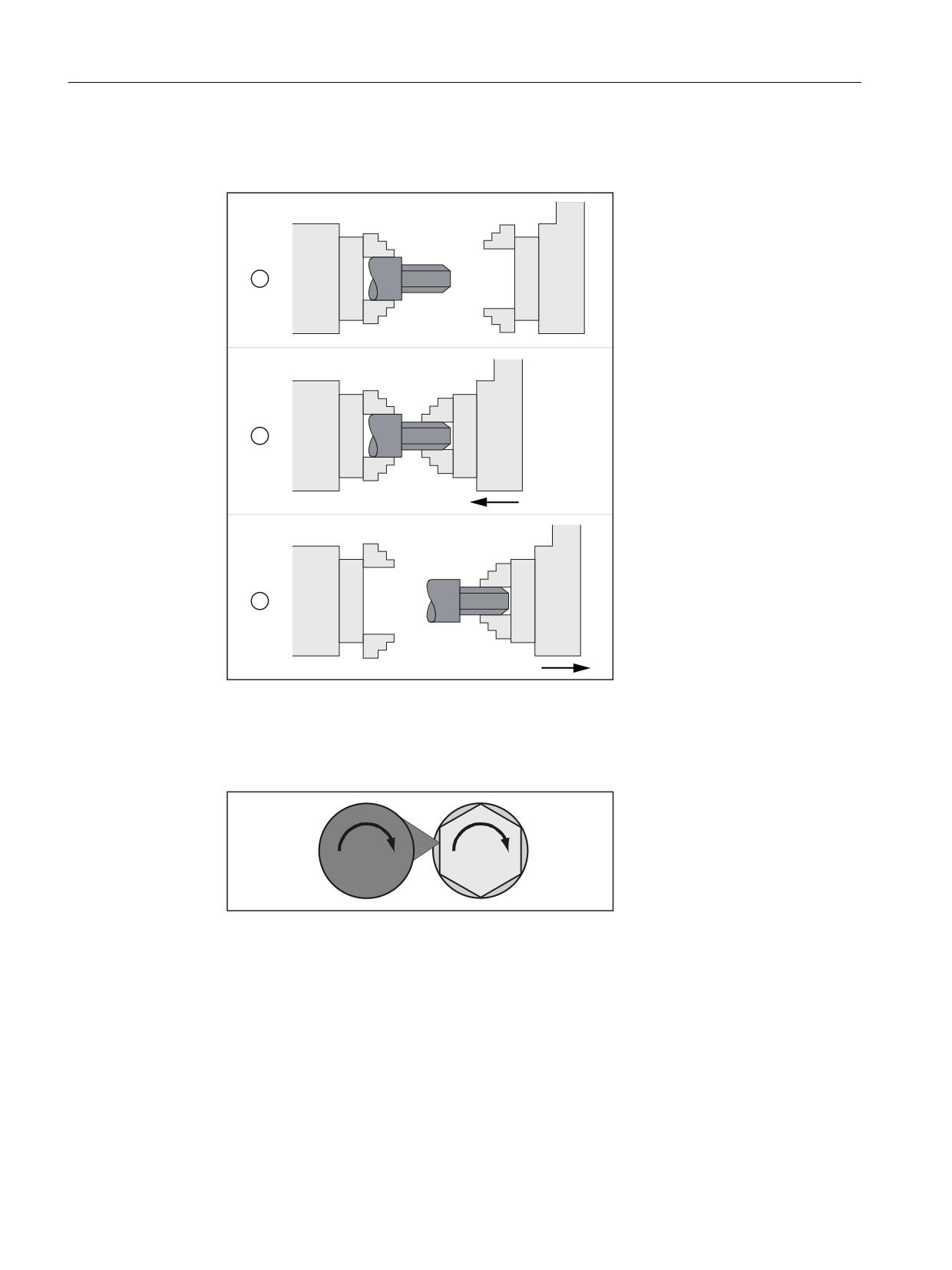
● Flying workpiece transfer, e.g. to machine the rear side, transformation ratio: 1:1
6
6
Q ำQ
6
6
Q
Q
6
6
Q ำQ
① Synchronize the speed
② Transfer the workpiece
③ Machine the rear side
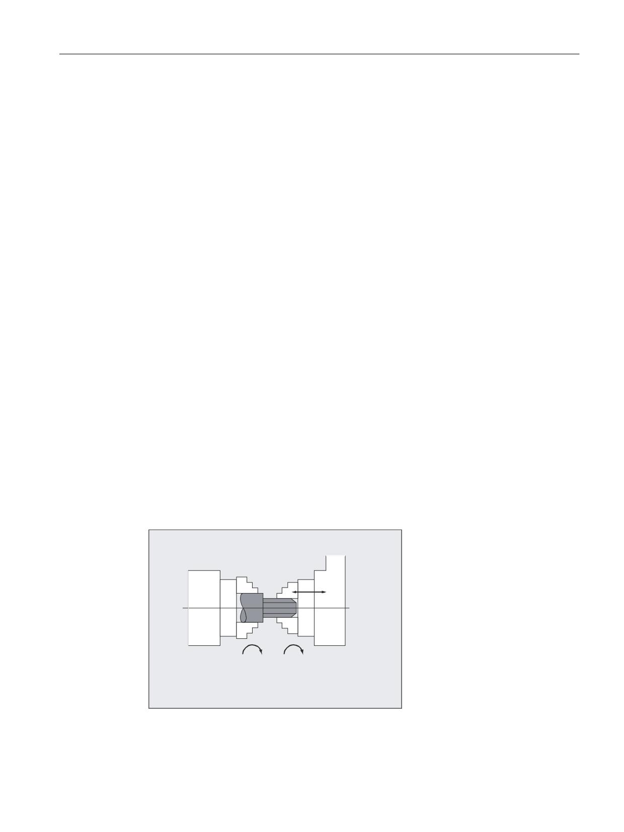
● Multi-edge machining (polygonal turning), speed synchronism, transformation ratio: n1:n2
Q
Q
Syntax
COUPDEF(<FS>,<LS>,<ZFS>,<NLS>,<block change>,<coupling type>)
COUPON(<FS>,<LS>,<POSFS>)
COUPONC(<FS>,<LS>)
COUPOF(<FS>,<LS>,<POSFS>,<POSLS>)
COUPOFS(<FS>,<LS>)
COUPOFS(<FS>,<LS>,<POSFS>)
COUPRES(<FS>,<LS>)
COUPDEL(<FS>,<LS>)
WAITC(<FS>,<block change>,<LS>,<block change>)
Job Planning
576
Programming Manual, 12/2018, A5E40869460B AB

Axis couplings
13.5 Synchronous spindle
Note
Abbreviated notation
A shorter notation without specification of the leading spindle is possible for the COUPOF,
COUPOFS, COUPRES and COUPDEL statements.
Meaning
COUPDEF:
Define/change coupling on user-specific basis
COUPON:
Activate coupling. The following spindle synchronizes to the leading spindle
based on the actual speed
COUPONC:
Coupling when activating with previous programming of M3 S... or
M4 S
A difference in speed for the following spindle is transferred immediately.
COUPOF:
Deactivate coupling.
● with immediate block change:
COUPOF(<S2>,<S1>)
● Block change only after <POSFS> or <POSLS> deactivation position(s) has
(have) been crossed:
COUPOF(<S2>,<S1>,<POSFS>)
COUPOF(<S2>,<S1>,<POSFS>,<POSLS>)
COUPOFS:
Deactivating a coupling with stop of following spindle.
Block change as quickly as possible with immediate block change:
COUPOFS(<S2>,<S1>)
Block change only after passing the switch-off position:
COUPOFS(<S2>,<S1>,<POSFS>)
COUPRES:
Reset coupling parameters to configured MD and SD
COUPDEL:
Delete user-defined coupling
WAITC:
Wait for synchronized run condition
(NOC are increased to IPO during block changes)
<FS>:
Designation of following spindle
Optional parameters:
<LS>:
Designation of main spindle
Specification with spindle number: e.g. S2, S1
<ZFS>, <NLS>:
Transformation ratio between FS and LS.
<ZFS>/<NLS> = numerator/denominator
Default setting: <ZFS> / <NLS> = 1.0 ; specification of denominator optional
Job Planning
Programming Manual, 12/2018, A5E40869460B AB
577

Axis couplings
13.5 Synchronous spindle
<block change>:
Block change behavior
The block change is:
"NOC"
Immediately
"FINE"
On reaching "Synchronism fine"
"COARSE"
On reaching "Synchronism coarse"
"IPOSTOP"
On reaching IPOSTOP; in other words, after setpoint-
based synchronism (default)
The block change behavior is effective modally.
<coupling type>:
Coupling type: Coupling between FS and LS
"DV"
Setpoint linkage (default)
"AV"
Actual value coupling
"VV"
Speed coupling
The coupling type is modal.
<POSFS>:
Angle offset between leading and following spindles
Range of val-
0°… 359.999°
ues:
<POSFS>,<POSLS>:
Switch-off positions of the following and leading spindles
"The block change is enabled once POSFS, POSLS has been passed"
Range of val-
0°… 359.999°
ues:
Examples
Working with leading and following spindles
Program code
Comment
Leading spindle = master spindle = spindle 1
Following spindle = spindle 2
N05 M3 S3000 M2=4 S2=500
Leading spindle rotates at 3000 rpm,
following spindle at 500 rpm.
N10 COUPDEF(S2,S1,1,1,"NOC","Dv")
Definition of the coupling (can also be config-
ured).
N70 SPCON
Bring leading spindle into closed-loop position
control (setpoint coupling).
N75 SPCON(2)
Bring following spindle into closed-loop posi-
tion control.
N80 COUPON(S2,S1,45)
On-the-fly coupling to offset position = 45 de-
grees.
N200 FA[S2]=100
Positioning speed = 100 degrees/min
N205 SPOS[2]=IC(-90)
Traverse with 90 degrees overlay in negative di-
rection.
N210 WAITC(S2,"Fine")
Wait for "fine" synchronism.
N212 G1 X... Y... F...
Machining
Job Planning
578
Programming Manual, 12/2018, A5E40869460B AB
Axis couplings
13.5 Synchronous spindle
Program code
Comment
N215 SPOS[2]=IC(180)
Traverse with 180 degrees overlay in the posi-
tive direction.
N220 G4 S50
Dwell time = 50 revolutions of the master spindle
N225 FA[S2]=0
Activate configured velocity (MD).
N230 SPOS[2]=IC(-7200)
20 revolutions. Move with configured velocity in
the negative direction.
N350 COUPOF(S2,S1)
Couple-out on-the-fly, S=S2=3000
N355 SPOSA[2]=0
Stop FS at zero degrees.
N360 G0 X0 Y0
N365 WAITS(2)
Wait for spindle 2.
N370 M5
Stop FS.
N375 M30
Programming a difference in speed
Program code
Comment
Leading spindle = master spindle = spindle 1
Following spindle = spindle 2
N01 M3 S500
Leading spindle rotates at 500 rpm.
N02 M2=3 S2=300
Following spindle rotates at 300 rpm.
N10 G4 F1
Dwell time of master spindle.
N15 COUPDEF (S2,S1,-1)
Coupling factor with ratio -1:1
N20 COUPON(S2,S1)
Activate coupling. The speed of the following
spindle results from the speed of the leading
spindle and coupling factor.
N26 M2=3 S2=100
Programming a difference in speed.
Examples of transfer of a movement for difference in speed
1. Activate coupling during previous programming of following spindle with COUPON
Program code
Comment
Leading spindle = master spindle = spindle 1
Following spindle = spindle 2
N05 M3 S100 M2=3 S2=200
Leading spindle rotates at 100 rpm, following
spindle at 200 rpm.
N10 G4 F5
Dwell time = 5 seconds of master spindle
N15 COUPDEF(S2,S1,1)
Transformation ratio of FS to LS is 1.0 (de-
fault).
N20 COUPON(S2,S1)
On-the-fly coupling to the leading spindle.
N10 G4 F5
Following spindle rotates at 100 rpm.
Job Planning
Programming Manual, 12/2018, A5E40869460B AB
579

Axis couplings
13.5 Synchronous spindle
2. Activate coupling during previous programming of following spindle with COUPONC
Program code
Comment
Leading spindle = master spindle = spindle 1
Following spindle = spindle 2
N05 M3 S100 M2=3 S2=200
Leading spindle rotates at 100 rpm, following
spindle at 200 rpm.
N10 G4 F5
Dwell time = 5 seconds of master spindle
N15 COUPDEF(S2,S1,1)
Transformation ratio of FS to LS is 1.0 (de-
fault).
N20 COUPONC(S2,S1)
On-the-fly coupling to leading spindle and trans-
fer previous speed to S2.
N10 G4 F5
S2 rotates at 100 rpm + 200 rpm = 300 rpm
3. Activate coupling with following spindle stationary with COUPON
Program code
Comment
Leading spindle = master spindle = spindle 1
Following spindle = spindle 2
N05 SPOS=10 SPOS[2]=20
Following spindle S2 in positioning mode.
N15 COUPDEF(S2,S1,1)
Transformation ratio of FS to LS is 1.0 (de-
fault).
N20 COUPON(S2,S1)
On-the-fly coupling to the leading spindle.
N10 G4 F1
Coupling is closed, S2 stops at 20 degrees.
4. Activate coupling with following spindle stationary with COUPONC
Note
Positioning or axis mode
If the following spindle is in positioning or axis mode before coupling, then the following spindle
behaves the same for COUPON(<FS>,<LS>) and COUPONC(<FS>,<LS>).
Note
Leading spindle and axis operation
If, prior to the coupling being defined, the leading spindle is in axis operation, the velocity limit
value from machine data
MD32000 $MA_MAX_AX_VELO (maximum axis velocity) will still apply even after the coupling
is activated.
To avoid this behavior, the axis must be switched to spindle mode (M3 S... or M4 S...)
prior to the coupling being defined.
Job Planning
580
Programming Manual, 12/2018, A5E40869460B AB
Axis couplings
13.5 Synchronous spindle
Further information
Configured coupling
For the configured coupling, the LS and FS are defined via machine data. The configured
spindles cannot be changed in the part program. The coupling can be parameterized in the
part program using COUPDEF (on condition that no write protection is valid).
User-defined coupling
COUPDEF can be used to redefine or change a coupling in the part program. If a coupling is
already active, it has to be deleted first with COUPDEL before a new coupling is defined.
A coupling is defined in its entirety by:
COUPDEF(<FS>,<LS>,<TFS>,<TLS>, block change behavior, coupling type)
Following spindle (FS) and leading spindle (LS)
The coupling is uniquely defined using the axis names for the FS and LS. The axis names
have to be programmed with every COUPDEF statement. The other coupling parameters are
modal and only have to be programmed if they change.
Example:
COUPDEF(S2,S1)
Transformation ratio
The transformation ratio is defined as the speed ratio between FS and LS:
Following spindle / leading spindle = numerator/denominator
The numerator must be programmed. The denominator must not be programmed. The default
value 1.0 is then set for the denominator.
Example:
Following spindle S2 and leading spindle S1, transformation ratio = 1/1
COUPDEF(S2, S1, 1.0)
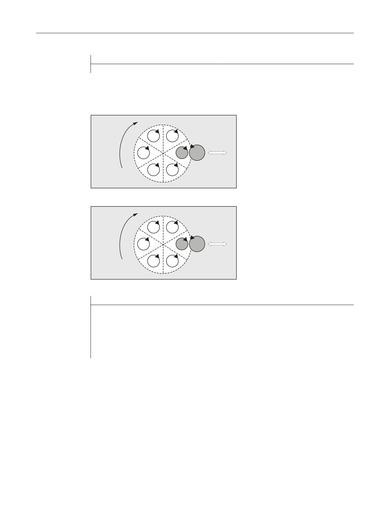
Q
Q
6SLQGOH
6SLQGOH
/HDG
)ROORZLQJ
VSLQGOH
VSLQGOH
Job Planning
Programming Manual, 12/2018, A5E40869460B AB
581
Axis couplings
13.5 Synchronous spindle
Note
The transformation ratio can also be changed on-the-fly (when the coupling is active and the
spindles are rotating).
Block change behavior NOC, FINE, COARSE, IPOSTOP
The following abbreviated notation can be used when programming the block change behavior:
● "NO": Immediately (default)
● "FI": On reaching "Synchronism fine"
● "CO": On reaching "Synchronism coarse"
● "IP": On reaching IPOSTOP; i.e. after setpoint-based synchronism
Type of coupling
Note
The coupling type may only be changed when the coupling is deactivated.
Activate synchronous mode COUPON, <POSFS>
● Activation of coupling with any angular offset between LS and FS:
- COUPON(S2,S1)
- COUPON(S2)
● Activation of coupling with angular offset <POSFS>
<POSFS> refers to the 0° position of the leading spindle in the positive direction of
rotation <POSFS> value range: 0°… 359,999°
- COUPON(S2,S1,30)
Note
The angular offset can also be changed when the coupling is active.
Position the following spindle
Even with activated synchronous spindle coupling, the FS can be positioned in the range ±180°
independently of the LS.
● Spindle positioning of the FS with SPOS
Example: SPOS[2]=IC(-90)
Further information on SPOS can be found in:
References:
Programming Manual, Fundamentals
Job Planning
582
Programming Manual, 12/2018, A5E40869460B AB
Axis couplings
13.5 Synchronous spindle
Differential speed
A speed difference results in speed control mode and active synchronous spindle coupling
through signed overlay of an FS speed because of LS movement and an FS speed because
of spindle programming:
● Synchronous spindle coupling with COUPONC
● S<FS>=<speed> [M<FS>=<direction of rotation>]
Note
Supplementary conditions
● Speed S... must also be reprogrammed with direction of rotation M3/M4.
● Overlay of a spindle speed (M<direction of rotation> S<FS>) through the LS
movement with synchronous spindle coupling COUPONC only becomes effective if the
overlay has been enabled.
● The dynamic responses of the leading spindle have to be restricted to such an extent
that when overlaying is applied to the following spindle, its dynamics limit values are not
exceeded.
For more information about the speed difference, see:
References:
Function Manual, Extended Functions; Synchronous Spindle (S3)
Velocity, acceleration: FA, ACC, OVRA, VELOLIMA
Axial velocity and acceleration of a following spindle can be programmed with:
● FA[SPI(S<n>)] or FA[S<n>] (axial velocity)
● ACC[SPI(S<n>)] or ACC[S<n>] (axial acceleration)
● OVRA[SPI(S<n>)] and OVRA[S<n>] (axial override)
● VELOLIMA[SPI(S<n>)] and VELOLIMA[S<n>] (increase and reduction of axial velocity
respectively)
When <n> = 1, 2, 3, ... (spindle numbers of the following spindles)
References:
Programming Manual, Fundamentals
Note
A reduction or increase of the maximum axial jerk has no effect with spindles.
Further information about the axial dynamic response is provided in:
References:
Function Manual, Extended Functions; Rotary Axes (R2)
Programmable block change behavior WAITC
WAITC can be used to define block change behavior, for example after a change to coupling
parameters or positioning actions, with a variety of synchronism conditions (coarse, fine,
IPOSTOP). If no synchronism conditions are specified, the block change behavior specified in
the COUPDEF definition will apply.
Job Planning
Programming Manual, 12/2018, A5E40869460B AB
583
Axis couplings
13.5 Synchronous spindle
Examples
● Wait for synchronism condition FINE to be fulfilled for following spindle S2 and COARSE to
be fulfilled for following spindle S4: WAITC(S2,"FINE",S4,"COARSE")
● Wait for synchronism condition according to COUPDEF to be fulfilled: WAITC( )
Deactivate coupling COUPOF
COUPOF can be used to define the turn-off behavior of the coupling:
● Deactivation of coupling with immediate block change:
- COUPOF(S2,S1) (with specification of leading spindle)
- COUPOF(S2) (without specification of leading spindle)
● Deactivation of coupling after switch-off positions have been crossed. The block change
takes place after the switch-off positions have been crossed.
- COUPOF(S2,S1,150) (switch-off position FS: 150°)
- COUPOF(S2,S1,150,30) (switch-off position FS: 150°, LS: 30°)
Deactivate coupling with following spindle stop COUPOFS
COUPOFS can be used to define the turn-off behavior of the coupling with following spindle stop:
● Deactivation of coupling with following spindle stop and immediate block change:
- COUPOFS(S2,S1) (with specification of leading spindle)
- COUPOFS(S2) (without specification of leading spindle)
● Deactivation of coupling after switch-off positions have been crossed with following spindle
stop. The block change takes place after the switch-off positions have been crossed.
- COUPOFS(S2,S1,150) (switch-off position FS: 150°)
Delete couplings COUPDEL
COUPDEL deletes the coupling:
● COUPDEL(S2,S1) (with specification of leading spindle)
● COUPDEL(S2) (without specification of leading spindle)
Reset coupling parameters, COUPRES
COUPRES activates the coupling values parameterized in the machine and setting data:
● COUPRES(S2,S1) (with specification of leading spindle)
● COUPRES(S2) (without specification of leading spindle)
System variables
● Current coupling status of following spindle
The current coupling status of a following spindle can be read bit-coded via:
<value> = $AA_COUP_ACT[<FS>]
Job Planning
584
Programming Manual, 12/2018, A5E40869460B AB
Axis couplings
13.5 Synchronous spindle
Bit
<value>
Meaning
-
0
No coupling active
2
4
Synchronous spindle coupling active
Note
● All other values refer to axis mode
● If the spindle is a following spindle or several couplings, then the value of the coupling state of all
couplings is returned as a total state.
● Current angular offset
The current angular offset of the following spindle to the leading spindle can be read via:
- $AA_COUP_OFFS[<FS>] (angular offset on the setpoint side)
- $VA_COUP_OFFS[<FS>] (angular offset on the actual value side)
Application example
Correction of the angular offset difference in the NC program after cancelling the follow-up
mode:
Angular offset difference = programmed angular offset - system variable
References
Detailed information on the system variables can be found in:
List Manual, System Variables
Job Planning
Programming Manual, 12/2018, A5E40869460B AB
585

Axis couplings
13.6 Generic coupling (CP...)
13.6
Generic coupling (CP...)
"Generic Coupling" is a general coupling function, combining all coupling characteristics of
existing coupling types (coupled motion, master value coupling, electronic gearbox and
synchronous spindle).
The function allows flexible programming:
● Users can select the coupling properties required for their applications (building block
principle).
● Each coupling property can be programmed individually.
● The coupling properties of a defined coupling (e.g. coupling factor) can be changed.
● Later use of additional coupling properties is possible.
● The coordinate reference system of the following axis (base coordinate system or machine
coordinate system) is programmable.
● Certain coupling properties can also be programmed with synchronous actions.
References: Function Manual, Synchronized Actions
Note
Previous coupling calls for coupled motion (TRAIL*), Master value coupling (LEAD*), Electronic
Gearbox (EG*) and Synchronous spindle (COUP*) are supported via adaptive cycles.
Overview of all keywords and coupling characteristics
The following table gives an overview of all keywords of the generic coupling and the
programmable coupling characteristics:
Keyword
Coupling characteristics / mean-
Syntax
ing
CPDEF
Creation of a coupling module
CPDEF=(<FAx>)
CPDEL
Deletion of a coupling module
CPDEL=(<FAx>)
CPLA
Definition of a leading axis
CPLA[<FAx>]=(<LAx>)
CPLDEF
Definition of a leading axis and
CPLDEF[<FAx>]=(<LAx>)
creation of a coupling module
or
(also possible with CPDEF +
CPDEF=(<FAx>) CPLA[<FAx>]=(<LAx>)
CPLA)
CPLDEL
Deletion of a leading axis of a
CPLDEL[<FAx>]=(<LAx>)
coupling module
or
(also possible with CPDEF +
CPDEL=(<FAx>) CPLA[<FAx>]=(<LAx>)
CPLA)
CPON
Switching on a coupling module
CPON=(<FAx>)
CPOF
Switching off a coupling module
CPOF=(<FAx>)
CPLON
Switching on a leading axis of a
CPLON[<FAx>]=<LAx>
coupling module
Job Planning
586
Programming Manual, 12/2018, A5E40869460B AB

Axis couplings
13.6 Generic coupling (CP...)
Keyword
Coupling characteristics / mean-
Syntax
ing
CPLOF
Switching off a leading axis of a
CPLOF[<FAx>]=<LAx>
coupling module
CPLNUM
Numerator of the coupling factor
CPLNUM[FAx,LAx]=<value>
CPLDEN
Denominator of the coupling
CPLDEN[FAx,LAx]=<value>
factor
CPLCTID
Number of the curve table
CPLCTID[FAx,LAx]=<value>
CPLSETVAL
Coupling reference
CPLSETVAL[FAx,LAx]="<coupling reference>"
"<coupling
"CMDPOS"
Setpoint value coupling
reference>":
"CMDVEL"
Speed coupling
"ACTPOS"
Actual value coupling
CPFRS
Coordinate reference system
CPFRS[FAx]="<coordinate reference>"
"<coordinate
"BCS"
Basic Coordinate System
reference>":
"MCS"
Machine Coordinate Sys-
tem
CPBC
Block change criterion
CPBC[FAx]="<block change criterion>"
"<block change
"NOC"
Block change is performed
criterion>":
irrespective of the coupling
status.
"IPOSTOP"
Block change is performed
with setpoint synchronism.
"COARSE"
Block change is performed
with actual value synchron-
ism “coarse”.
"FINE"
Block change is performed
with actual value synchron-
ism "fine".
CPFPOS + CPON
Synchronized position of the fol-
CPON=FAx CPFPOS[FAx]=<value>
lowing axis when switching on
CPLPOS + CPON
Synchronized position of the
CPLPOS[FAx,LAx]=<value>
leading axis when switching on
Job Planning
Programming Manual, 12/2018, A5E40869460B AB
587

Axis couplings
13.6 Generic coupling (CP...)
Keyword
Coupling characteristics / mean-
Syntax
ing
CPFMSON
Synchronization mode
CPFMSON[FAx]="<synchronization mode>"
"<synchronization
"CFAST"
The coupling is closed time-
mode>":
optimized.
"CCOARSE"
The coupling is only closed
when the following axis po-
sition, required according
to the coupling rule, is in the
range of the current follow-
ing axis position.
"NTGT"
The next tooth gap is ap-
proached time-optimized.
"NTGP"
The next tooth gap is ap-
proached path-optimized.
"NRGT"
The next segment is ap-
proached in a time-opti-
mized manner, in accord-
ance with the ratio of the
number of gears to the
number of teeth.
"NRGP"
The next segment is ap-
proached in a path-opti-
mized manner, in accord-
ance with the ratio of the
number of gears to the
number of teeth.
"ACN"
For rotary axes only!
The rotary axis traverses to
the synchronized position
in the negative axis direc-
tion. Synchronization is re-
alized immediately.
"ACP"
For rotary axes only!
The rotary axis traverses to
the synchronized position
in the positive axis direc-
tion. Synchronization is re-
alized immediately.
"DCT"
For rotary axes only!
The rotary axis traverses to
the programmed synchron-
ized position time-opti-
mized. Synchronization is
realized immediately.
"DCP"
For rotary axes only!
The rotary axis traverses to
the programmed synchron-
ized position path-opti-
mized. Synchronization is
realized immediately.
Job Planning
588
Programming Manual, 12/2018, A5E40869460B AB

Axis couplings
13.6 Generic coupling (CP...)
Keyword
Coupling characteristics / mean-
Syntax
ing
CPFMON
Behavior of the following axis
CPFMON[FAx]= "<switch-on behavior>"
when switching on
"<switch-on
"STOP"
For spindles only!
behavior>":
An active motion of the fol-
lowing spindle is stopped
before switch-on.
"CONT"
For spindles and main tra-
verse axes only!
The current motion of the
following axis/spindle is tak-
en over into the coupling as
start motion.
"ADD"
For spindles only!
The motion components of
the coupling operate in ad-
dition to the currently over-
laid motion, i.e. the current
motion of the following axis/
spindle is retained as over-
laid motion.
CPFMOF
Behavior of the following axis at
CPFMOF[FAx]="<switch-off behavior>"
complete switch-off
"<switch-off
"STOP"
Stop of a following axis/
behavior>":
spindle.
An active overlaid motion is
also braked to standstill.
The coupling is then
opened
"CONT"
For spindles and main tra-
verse axes only!
The following spindle con-
tinues to traverse at the
speed/velocity that applied
at the instant of deactiva-
tion.
CPFPOS + CPOF
Switch-off position of the follow-
CPOF=(FAx) CPFPOS[FAx]=<value>
ing axis when switching off
Job Planning
Programming Manual, 12/2018, A5E40869460B AB
589

Axis couplings
13.6 Generic coupling (CP...)
Keyword
Coupling characteristics / mean-
Syntax
ing
CPMRESET
Coupling behavior for RESET
CPMRESET[FAx]="<Reset behavior>"
"<reset
"NONE"
The current state of the cou-
behavior>":
pling is retained.
"ON"
When the appropriate cou-
pling module is created, the
coupling is switched on. All
defined leading axis rela-
tionships are activated.
This is also performed
when all or parts of these
leading axis relationships
are active, i.e. resynchroni-
zation is performed even
with a completely activated
coupling.
"OF"
An active overlaid motion is
also braked to standstill.
The coupling is then deacti-
vated. When the relevant
coupling module was cre-
ated without an explicit def-
inition (CPDEF), the cou-
pling module is deleted.
Otherwise it is retained, i.e.
it can still be used.
"OFC"
Possible only in spindles!
The following spindle con-
tinues to traverse at the
speed/velocity that applied
at the instant of deactiva-
tion. The coupling is switch-
ed off. When the relevant
coupling module was cre-
ated without an explicit def-
inition (CPDEF), the cou-
pling module is deleted.
Otherwise it is retained, i.e.
it can still be used.
"DEL"
An active overlaid motion is
also braked to standstill.
The coupling is then deacti-
vated and then deleted.
"DELC"
Possible only in spindles!
The following spindle con-
tinues to traverse at the
speed/velocity that applied
at the instant of deactiva-
tion. The coupling is deacti-
vated and then deleted.
Job Planning
590
Programming Manual, 12/2018, A5E40869460B AB

Axis couplings
13.6 Generic coupling (CP...)
Keyword
Coupling characteristics / mean-
Syntax
ing
CPMSTART
Coupling behavior at part pro-
CPMSTART[FAx]="<start behavior>"
gram start
"<start
"NONE"
The current state of the cou-
behavior>":
pling is retained.
"ON"
Coupling switched-on. All
defined leading axis rela-
tionships are activated.
This is also performed
when all or parts of these
leading axis relationships
are active, i.e. resynchroni-
zation is performed even
with a completely activated
coupling.
"OF"
The coupling is switched
off. When the relevant cou-
pling module was created
without an explicit definition
(CPDEF), the coupling
module is deleted. Other-
wise it is retained, i.e. it can
still be used.
"DEL"
The coupling is deactivated
and then deleted.
CPMPRT
Coupling response at part pro-
CPMPRT[FAx]="<start behavior>"
gram start under block search
"<start
see CPMSTART
run via program test
behavior>":
CPLINTR
Offset value of the input value
CPLINTR[FAx,LAx]=<value>
of a leading axis
CPLINSC
Scaling factor of the input value
CPLINSC[FAx,LAx]=<value>
of a leading axis
CPLOUTTR
Offset value for the output value
CPLOUTTR[FAx,LAx]=<value>
of a coupling
CPLOUTSC
Scaling factor for the output val-
CPLOUTSC[FAx,LAx]=<value>
ue of a coupling
CPSYNCOP
Threshold value of position syn-
CPSYNCOP[FAx]=<value>
chronism "Coarse"
CPSYNFIP
Threshold value of position syn-
CPSYNFIP[FAx]=<value>
chronism "Fine"
CPSYNCOP2
Second threshold value for the
CPSYNCOP2[FAx]=<value>
"Coarse" position synchronism
CPSYNFIP2
Second threshold value for the
CPSYNFIP2[FAx]=<value>
"Fine" position synchronism
CPSYNCOV
Threshold value of velocity syn-
CPSYNCOV[FAx]=<value>
chronism "Coarse"
CPSYNFIV
Threshold value of velocity syn-
CPSYNFIV[FAx]=<value>
chronism "Fine"
Job Planning
Programming Manual, 12/2018, A5E40869460B AB
591

Axis couplings
13.6 Generic coupling (CP...)
Keyword
Coupling characteristics / mean-
Syntax
ing
CPMBRAKE
Response of the following axis
CPMBRAKE[FAx]=<bit-coded value>
to certain stop signals and stop
commands
CPMVDI
Response of the following axis
CPMVDI[FAx]=<bit-coded value>
to certain NC/PLC interface sig-
nals
CPMALARM
Suppression of special cou-
CPMALARM[FAx]=<bit-coded value>
pling-related alarm outputs
CPSETTYPE
Coupling type
CPSETTYPE[FAx]="<coupling type>"
"<coupling type>":
"CP"
Freely programmable
"TRAIL"
Coupling type "Coupled
motion"
"LEAD"
Coupling type "Master Val-
ue Coupling"
"EG"
Coupling type "Electronic
gearbox"
"COUP"
Coupling type "Synchron-
ized spindle"
FAx: Following axis/spindle
LAx: Leading axis/spindle
Note
Coupling characteristics, which are not explicitly programmed (in part program of synchronous
actions), become effective with their default settings.
Depending on the settings of the keyword CPSETTYPE instead of the default settings
(CPSETTYPE="CP") preset coupling characteristics can become effective.
References
For detailed information on generic couplings, see:
● Function Manual, Special Functions; M3: Axis couplings, Chapter: "Generic coupling"
Job Planning
592
Programming Manual, 12/2018, A5E40869460B AB

Axis couplings
13.7 Master/slave coupling (MASLDEF, MASLDEL, MASLON, MASLOF, MASLOFS)
13.7
Master/slave coupling (MASLDEF, MASLDEL, MASLON, MASLOF,
MASLOFS)
The "master/slave coupling" enables:
● The coupling of the slave axes to the master axis, when the axes involved are at standstill.
● The coupling/decoupling of rotating, speed-controlled spindles.
● The dynamic configuration.
Note
Positioning mode
For axes and spindles in the positioning mode, the coupling is only closed and opened at
standstill.
Syntax
MASLON(<slave_1>,<slave_2>,...)
MASLOF(<slave_1>,<slave_2>,...)
MASLOFS(<slave_1>,<slave_2>,...)
Dynamic configuration:
MASLDEF(<slave_1>,<slave_2>, ... ,<master>)
MASLDEL(<slave_1>,<slave_2>,...)
Meaning
MASLON:
Activating a temporary master/slave coupling
<Slave_x>,...:
Slave axis 1 ... n
MASLOF:
Decoupling an active master/slave coupling
<slave_1>,...:
Slave axis 1 ... n
MASLOFS:
Decoupling a master/slave coupling and automatically braking slave spindles (see note
"Coupling behavior for spindles! in speed control mode"!)
<slave_1>,...:
Slave axis 1 ... n
MASLDEF:
Creating/changing a master/slave group from the part program
<slave_1>,...:
Slave axis 1 ... n
<master>:
Master axis
MASLDEL:
Separate master/slave coupling and delete the definition of the grouping
<slave_1>,...:
Slave axis 1 ... n
Note:
The master/slave definitions configured in the machine data are retained.
Job Planning
Programming Manual, 12/2018, A5E40869460B AB
593

Axis couplings
13.7 Master/slave coupling (MASLDEF, MASLDEL, MASLON, MASLOF, MASLOFS)
Note
Coupling behavior for spindles in speed control mode
For spindles in the speed control mode, the coupling behavior of MASLON, MASLOF, MASLOFS
and MASLDEL are specified explicitly via the following machine data:
MD37263 $MA_MS_SPIND_COUPLING_MODE
For the default setting with MD37263 = 0, the slave axes are coupled-in and coupled-out only
when the axes involved are at standstill. MASLOFS corresponds to MASLOF.
For MD37263 = 1, the coupling instruction is immediately executed and therefore also the
motion. For MASLON the coupling is immediately closed and for MASLOFS or MASLOF
immediately opened. With MASLOF, the slave spindles rotating at this instant keep their speeds
until a new speed is programmed. However, with MASLOFS, they are braked automatically.
Note
For MASLOF/MASLOFS, the implicit preprocessing stop is not required. Because of the missing
preprocessing stop, the $P system variables for the slave axes do not provide updated values
until next programming.
Note
For the slave axis, the actual value can be synchronized to the same value of the master axis
using PRESETON. To do this, the permanent/slave coupling must be briefly switched off in order
to set the actual value of the non-referenced slave axis to the value of the master/axis with
POWER ON. Then the coupling is permanently re-established.
The permanent master/slave coupling is activated with the following MD setting:
MD37262 $MA_MS_COUPLING_ALWAYS_ACTIVE = 1
It has no effect on the language commands of the temporary coupling.
Examples
Example 1: Set actual value for the slave axis of a master/slave coupling
For a permanent master/slave coupling, PRESETON sets the actual value of the slave axis to
the value of the master axis.
Program code
Comment
$MA_MS_COUPLING_ALWAYS_ACTIVE[AX2]=0
; Deactivate the permanent coupling of
the slave axis
NEWCONF
; Activate machine data change
STOPRE
MASLOF(Y1)
; Deactivate temporary coupling
PRESETON(AX2,$VA_IM(M_AX))
; Actual value of the slave axis = actual
value of the master axis
$MA_MS_COUPLING_ALWAYS_ACTIVE[AX2]=1
; Activate the permanent coupling of the
slave axis
Job Planning
594
Programming Manual, 12/2018, A5E40869460B AB
Axis couplings
13.7 Master/slave coupling (MASLDEF, MASLDEL, MASLON, MASLOF, MASLOFS)
Program code
Comment
NEWCONF
; Activate machine data change
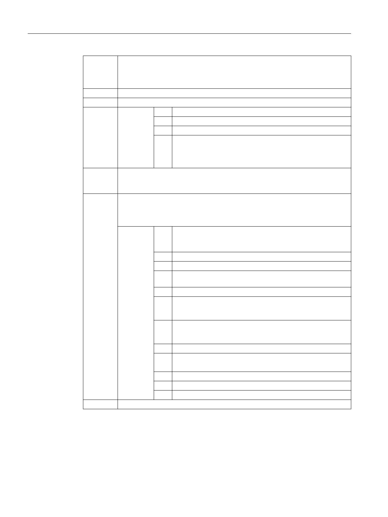
Example 2: Dynamic configuration of a master/slave coupling
To enable coupling with another spindle after axis container rotation, the previous coupling
must be uncoupled, the configuration cleared, and a new coupling configured.
6
6
'LUHFWLRQ RI
URWDWLRQ
$;
$;
0HFKDQLFDO
FRQWDLQHU
LQIHHG
6
$;
$;
$8;
$;
$;
6
6
Figure 13-1
Prior to the axis container rotation
6
6
'LUHFWLRQ RI
URWDWLRQ
$;
$;
0HFKDQLFDO
FRQWDLQHU
LQIHHG
6
$;
$;
$8;
$;
$;
6
6
Figure 13-2
After axis container rotation by one slot
Program code
Comment
MASLDEF(AUX,S3)
; AUX: Slave, S3: Master = AX3
MASLON(AUX)
; Coupling on
M3=3 S3=4000
; Rotate master
MASLDEL(AUX)
; Disconnect and delete coupling
AXCTSWE(CT1)
; Enable axis container rotation
MASLDEF(AUX,S3)
; AUX: Slave, S3: Master = AX2
References
● Function Manual Special Functions, Chapter "TE3: Speed/torque coupling, master-slave"
● Function Manual Extended Functions, Chapter "B3: Distributed systems - only 840D sl" >
"NCU link" > "Axis container"
Job Planning
Programming Manual, 12/2018, A5E40869460B AB
595
Axis couplings
13.7 Master/slave coupling (MASLDEF, MASLDEL, MASLON, MASLOF, MASLOFS)
Job Planning
596
Programming Manual, 12/2018, A5E40869460B AB
Synchronized actions
14
14.1
Definition of a synchronized action
A synchronized action is defined in a block of a part program. Any further commands that are
not part of the synchronized action, may not be programmed within this block.
A synchronized action consists of the following components:
Validity, ID no.
Condition part
Action part
(optional)
(optional)
Frequency
G command
Condition
Keyword
G command
Actions
(optional)
(optional)
--- 1)
--- 1)
G...
Logical expres-
DO
G...
Action 1
sion
ID=<no.>
WHENEVER
IDS=<no.>
FROM
Action n
WHEN
EVERY
1)
Not programmed
Syntax
DO <action 1> ... <action n>
<frequency> [<G function>] <condition> DO <action 1> ... <action n>
ID=<No> <frequency> [<G function>] <condition> DO <action 1> ...
<action n>
IDS=<No> <frequency> [<G function>] <condition> DO <action 1> ...
<action n>
References
A detailed description of the functionality of synchronized actions can be found in:
Function Manual, Synchronized Actions
Job Planning
Programming Manual, 12/2018, A5E40869460B AB
597
Synchronized actions
14.1 Definition of a synchronized action
Job Planning
598
Programming Manual, 12/2018, A5E40869460B AB
Oscillation
15
15.1
Asynchronous oscillation (OS, OSP1, OSP2, OST1, OST2, OSCTRL,
OSNSC, OSE, OSB)
An oscillating axis travels back and forth between two reversal points 1 and 2 at a defined
feedrate, until the oscillating motion is deactivated.
Other axes can be interpolated as desired during the oscillating motion. A continuous infeed
can be achieved via a path movement or with a positioning axis, however, there is no
relationship between the oscillating movement and the infeed movement.
Properties of asynchronized oscillation
● Asynchronous oscillation is active on an axis-specific basis beyond block limits.
● Block-oriented activation of the oscillation movement is ensured by the part program.
● Combined interpolation of several axes and superimposing of oscillation paths are not
possible.
Programming
The following commands can be used to activate and control asynchronous oscillation from
the part program.
The programmed values are entered in the corresponding setting data with block
synchronization during the main run and remain active until changed again.
Syntax
OSP1[<axis>]=<value> OSP2[<axis>]=<value>
OST1[<axis>]=<value> OST2[<axis>]=<value>
FA[<axis>]=<value>
OSCTRL[<axis>]=(<setting option>,<reset option>)
OSNSC[<axis>]=<value>
OSE[<axis>]=<value>
OSB[<axis>]=<value>
OS[<axis>] = 1
OS[<axis>] = 0
Meaning
<axis>:
Name of oscillating axis
OS:
Activate/deactivate oscillation
Value:
1
Switch oscillation on
0
Switch oscillation off
OSP1:
Define position of reversal point 1
Job Planning
Programming Manual, 12/2018, A5E40869460B AB
599
Oscillation
15.1 Asynchronous oscillation (OS, OSP1, OSP2, OST1, OST2, OSCTRL, OSNSC, OSE, OSB)
OSP2:
Define position of reversal point 2
Note:
If incremental movement is active, the position will be calculated incrementally to the last
corresponding reversal position programmed in the NC program.
OST1:
Define stopping time in reversal point 1 in [s]
OST2:
Define stopping time in reversal point 2 in [s]
<value>:
-2
Interpolation continues without wait for exact stop
-1
Wait for exact stop coarse
0
Wait for exact stop fine
>0
Wait for exact stop fine and then wait for specified stopping time
Note:
The unit for the stopping time is identical to that of the stopping time
programmed with G4.
FA:
Define feedrate
The feedrate is the defined feedrate of the positioning axis. If no feedrate is defined, the
value stored in the machine data applies.
OSCTRL:
Specify setting and reset options
Option values 0 to 3 encrypt the behavior at the reversal points on deactivation. One of
the variants from 0 to 3 can be selected. The remaining settings can be combined at will
with the selected variant. Multiple options are appended with plus characters (+).
<value>:
0
Stop at next reversal point on deactivation of oscillation (default)
Note:
Only possible if values 1 and 2 are reset.
1
When the oscillation is deactivated, stop at reversal point 1
2
When the oscillation is deactivated, stop at reversal point 2
3
When the oscillation is deactivated, do not approach reversal point
if no spark-out strokes are programmed
4
Approach end position after spark-out
8
If oscillation is canceled by deletion of distance-to-go, sparking-out
strokes will then need to be executed and the end position approach-
ed if necessary.
16
If oscillation is canceled by deletion of distance-to-go, the corre-
sponding reversal point will need to be approached as is the case
with shutdown.
32
New feed is only active after the next reversal point
64
FA equal to 0, FA = 0: Path overlay is active
FA not equal to 0, FA <> 0: Speed overlay is active
128
For rotary axis DC (shortest path)
256
The sparking-out stroke is a dual stroke (default). 1=Single stroke.
512
First approach start position
OSNSC:
Define number of sparking-out strokes
Job Planning
600
Programming Manual, 12/2018, A5E40869460B AB

Oscillation
15.1 Asynchronous oscillation (OS, OSP1, OSP2, OST1, OST2, OSCTRL, OSNSC, OSE, OSB)
OSE:
Define end position (in workpiece coordinate system) to be approached after deactivation
of oscillation.
Note:
When programming "OSE" option 4 becomes effective implicitly for "OSCTRL".
OSB:
Define start position (in workpiece coordinate system) to be approached prior to activation
of oscillation.
The start position is approached before reversal point 1. If the start position coincides with
reversal position 1, reversal position 2 is approached next. No stopping time applies when
the start position is reached, even if this position coincides with reversal position 1; in-
stead, the axis waits for the exact stop fine signal. Any exact stop condition configured is
fulfilled.
Note:
Bit 9 in setting data SD43770 $SA_OSCILL_CTRL_MASK must be set to initiate an ap-
proach to the start position.
Examples
Example 1: Oscillating axis to oscillate between two reversal points
Oscillating axis Z is to oscillate between position 10 and 100. Reversal point 1 is to be
approached with exact stop fine, reversal point 2 with exact stop coarse. The feedrate for the
oscillating axis must be 250. 3 sparking-out strokes must be executed at the end of the
machining operation and the oscillating must approach end position 200. The feedrate for the
infeed axis must be 1 and the end of infeed in the X direction should be reached at position
15.
Program code
Comment
WAITP(X,Y,Z)
; Initial setting.
G0 X100 Y100 Z100
; Switch over to positioning axis opera-
tion.
WAITP(X,Z)
OSP1[Z]=10 OSP2[Z]=100
; Reversal point 1, reversal point 2.
OSE[Z]=200
; End position.
OST1[Z]=0 OST2[Z]=-1
;Stopping time at U1: Exact stop fine
; Stopping time at U2: Exact stop coarse
FA[Z]=250 FA[X]=1
; Feed for oscillating axis, infeed axis
OSCTRL[Z]=(4,0)
; Setting options.
OSNSC[Z]=3
; 3 sparking-out strokes.
OS[Z]=1
; Start oscillation.
WHEN $A_IN[3]==TRUE DO DELDTG(X)
; Deletion of distance-to-go.
POS[X]=15
; Starting position X axis.
POS[X]=50
; End position X axis.
OS[Z]=0
; Stop oscillation.
M30
Note
The "OSP1[Z]=..." to "OSNCS[Z]=..." command sequence can also be programmed in a block.
Job Planning
Programming Manual, 12/2018, A5E40869460B AB
601
Oscillation
15.1 Asynchronous oscillation (OS, OSP1, OSP2, OST1, OST2, OSCTRL, OSNSC, OSE, OSB)
Example 2: Oscillation with online modification of the reversal position
The setting data necessary for asynchronous oscillation can be set in the part program.
If the setting data is described directly in the program, the change takes effect during
preprocessing. A synchronized response can be achieved by means of a preprocessing stop
(STOPRE).
Program code
Comment
$SA_OSCILL_REVERSE_POS1[Z]=-10
$SA_OSCILL_REVERSE_POS2[Z]=10
G0 X0 Z0
WAITP(Z)
ID=1 WHENEVER $AA_IM[Z] < $$AA_OSCILL_REVERSE_
; If the actual value of the os-
POS1[Z] DO $AA_OVR[X]=0
cillating axis has exceeded the
reversal point, then the infeed
ID=2 WHENEVER $AA_IM[Z] < $$AA_OSCILL_REVERSE_
axis is stopped.
POS2[Z] DO $AA_OVR[X]=0
OS[Z]=1 FA[X]=1000 POS[X]=40
; Activate oscillation.
OS[Z]=0
; Deactivate oscillation.
M30
Further information
Oscillating axis
The following apply to the oscillating axis:
● Every axis may be used as an oscillation axis.
● Several oscillation axes can be active at the same time (maximum: the number of the
positioning axes).
● Linear interpolation G1is always active for the oscillating axis - irrespective of the G
command currently valid in the program.
The oscillating axis can:
● Act as an input axis for dynamic transformation
● Act as a guide axis for gantry and coupled-motion axes
● Be traversed:
- Without jerk limitation "BRISK"
or
- With jerk limitation "SOFT"
or
- With acceleration curve with a knee (as positioning axes)
Job Planning
602
Programming Manual, 12/2018, A5E40869460B AB
Oscillation
15.1 Asynchronous oscillation (OS, OSP1, OSP2, OST1, OST2, OSCTRL, OSNSC, OSE, OSB)
Oscillation reversal points
The current offsets must be taken into account when oscillation positions are defined:
● Absolute specification
"OSP1[Z]=<value>"
Position of reversal point = sum of offsets + programmed value
● Relative specification
"OSP1[Z]=IC(<value>)"
Position of reversal point = reversal point 1 + programmed value
Example:
Program code
N10 OSP1[Z]=100 OSP2[Z]=110
N40 OSP1[Z]=IC(3)
WAITP
If oscillation is to be performed with a geometry axis, you must enable this axis for oscillation
with "WAITP".
When oscillation has finished, "WAITP" is used to enter the oscillating axis as a positioning
axis again, so that normal use can resume.
Oscillation with motion-synchronous actions and stopping times
Once the set stop times have expired, the internal block change is executed during oscillation
(indicated by the new distances to go of the axes). The deactivation function is checked when
the block changes. The deactivation function is defined according to the control setting for the
motion sequence (OSCTRL). This dynamic response can be influenced by the feed override.
An oscillation stroke may then be executed before the sparking-out strokes are started or the
end position approached. Although it appears as if the deactivation response has changed,
this is not in fact the case.
Job Planning
Programming Manual, 12/2018, A5E40869460B AB
603

Oscillation
15.2 Oscillation controlled by synchronized actions (OSCILL)
15.2
Oscillation controlled by synchronized actions (OSCILL)
With this mode of oscillation, an infeed motion may only be executed at the reversal points or
within defined reversal areas.
Depending on requirements, the oscillation movement can be
● Continued or
● Stopped until the infeed has finished executing.
Syntax
1. Define parameters for oscillation
2. Define motion-synchronous actions
3. Assign axes, define infeed
Meaning
OSP1[<oscillating axis>]=
Position of reversal point 1
OSP2[<oscillating axis>]=
Position of reversal point 2
OST1[<oscillating axis>]=
Stopping time at reversal point 1 in seconds
OST2[<oscillating axis>]=
Stopping time at reversal point 2 in seconds
FA[<oscillating axis>]=
Feed for oscillating axis
OSCTRL[<oscillating axis>]=
Set or reset options
OSNSC[<oscillating axis>]=
Number of sparking-out strokes
OSE[<oscillating axis>]=
End position
WAITP(<oscillating axis>)
Enable axis for oscillation
Axis assignment, infeed
OSCILL[<oscillating axis>]=(<infeed axis 1>,<infeed axis 2>,<infeed
axis 3>)
POSP[<infeed axis>]=(<end position>,<partial length>,<mode>)
OSCILL:
Assign infeed axis or axes for oscillating axis
POSP:
Define complete and partial infeeds (see Section "File and Program Management")
End position:
End position for the infeed axis after all partial infeeds have been traversed.
Partial
Length of the partial infeed at reversal point/reversal area
length:
Mode:
Division of the complete infeed into partial infeeds
= Two residual steps of equal size (default);
= All partial infeeds of equal size
Motion-synchronous actions
WHEN… … DO
when…, do…
WHENEVER … DO
whenever…, do…
Job Planning
604
Programming Manual, 12/2018, A5E40869460B AB

Oscillation
15.2 Oscillation controlled by synchronized actions (OSCILL)
Example
No infeed must take place at reversal point 1. At reversal point 2, the infeed is to start at a
distance of ii2 before reversal point 2 and the oscillating axis is not to wait at the reversal point
for the end of the partial infeed. Axis Z is the oscillation axis and axis X the infeed axis.
=
$SSURDFK UHYHUVDO SRVLWLRQ
$SSURDFK HQG
DQG VSDUNLQJ RXW VWURNHV
SRVLWLRQ
;
1. Parameters for oscillation
Program code
Comment
DEF INT ii2
; Define variable for reversal area 2
OSP1[Z]=10 OSP2[Z]=60
; Define reversal points 1 and 2
OST1[Z]=0 OST2[Z]=0
; Reversal point 1: Exact stop fine
Reversal point 2: Exact stop fine
FA[Z]=150 FA[X]=0.5
; Oscillating axis Z feedrate, infeed axis X feedrate
OSCTRL[Z]=(2+8+16.1)
; Deactivate oscillating motion at reversal point 2; after
delete DTG spark-out and approach end position; after de-
lete DTG approach reversal position
OSNC[Z]=3
; Sparking-out strokes
OSE[Z]=70
; End position = 70
ii2=2
; Set reversal point range
WAITP(Z)
; Enable oscillation for Z axis
2. Synchronized action
Program code
Comment
WHENEVER $AA_IM[Z]<$SA_OSCILL_REVERSE_POS2[Z]
; If the actual position of oscil-
DO ->
lating axis Z in MCS is less than
$AA_OVR[X]=0 $AC_MARKER[0]=0
the start of reversal range 2, then
always set the axial override of the
infeed axis X to 0% and the bit mem-
ory with index 0 to the value 0.
Job Planning
Programming Manual, 12/2018, A5E40869460B AB
605
Oscillation
15.2 Oscillation controlled by synchronized actions (OSCILL)
Program code
Comment
WHENEVER $AA_IM[Z]>=$SA_OSCILL_REVERSE_POS2[Z]
; If the actual position of the os-
DO $AA_OVR[Z]=0
cillating axis Z in MCS is greater
than the reversal position 2, then
always set the axial override of the
oscillating axis Z to 0%.
WHENEVER $AA_DTEPW[X] == 0 DO $AC_MARKER[0]=1
; If the remaining distance to go of
the partial infeed is 0, then always
set the bit memory with index 0 to
the value 1.
WHENEVER $AC_MARKER[0]==1 DO $AA_OVR[X]=0
; Whenever the bit memory with index
$AA_OVR[Z]=100
0 is equal to 1, then set the axial
override of the infeed axis X to 0%.
As a consequence, a premature infeed
is prevented (oscillating axis Z has
still not left reversal area 2, but
infeed axis X is ready for a new in-
feed). Set the axial override of os-
cillating axis Z from 0% (action of
the 2nd synchronized action) back to
100% to move.
-> must be programmed in a single block
3. Start oscillation
Program code
Comment
OSCILL[Z]=(X) POSP[X]=(5,1,1)
; Start the axes
Oscillating axis Z is assigned ax-
is X as infeed axis.
Up to end position 5, axis X
should travel in steps of 1.
M30
; End of program
Further information
1. Define oscillation parameters
The parameters for oscillation should be defined before the movement block containing the
assignment of infeed and oscillating axes and the infeed definition (see "Asynchronized
oscillation").
2. Define motion-synchronized actions
The following synchronization conditions can be defined:
Suppress infeed until the oscillating axis is located within a reversal area
(ii1, ii2) or at a reversal point (U1, U2).
Stop oscillation motion during infeed at reversal point.
Restart oscillation movement on completion of partial infeed. Define
start of next partial infeed.
3. Assign oscillating and infeed axes as well as partial and complete infeed.
Job Planning
606
Programming Manual, 12/2018, A5E40869460B AB

Oscillation
15.2 Oscillation controlled by synchronized actions (OSCILL)
Define oscillation parameters
Assignment of oscillating and infeed axes: OSCILL
OSCILL[<oscillating axis>]=(<infeed axis1>,<infeed axis2>,<infeed
axis3>)
The axis assignments and the start of the oscillation movement are defined with the "OSCILL"
command.
Up to 3 infeed axes can be assigned to an oscillating axis.
Note
Before oscillation starts, the synchronization conditions must be defined for the behavior of
the axes.
Define infeeds: POSP
POSP[<infeed axis>]=(<end position>,<partial length>,<mode>)
The following are declared to the control with the "POSP" command:
● Complete infeed (with reference to end position)
● The length of the partial infeed at the reversal point or in the reversal area
● The partial infeed response when the end position is reached (with reference to mode)
Mode = 0
The distance-to-go to the destination point for the last two partial infeeds is divided
into two equal steps (default setting).
Mode = 1
All partial infeeds are of equal size. They are calculated from the complete infeed.
Define motion-synchronized actions
The synchronized-motion actions listed below are used for general oscillation.
You are given example solutions for individual tasks, which you can use as modules for creating
user-specific oscillation movements
Note
In individual cases, the synchronization conditions can be programmed differentially.
Keywords
WHEN … DO …
when…, do…
WHENEVER … DO
whenever…, do…
Job Planning
Programming Manual, 12/2018, A5E40869460B AB
607
Oscillation
15.2 Oscillation controlled by synchronized actions (OSCILL)
Functions
You can implement the following functions with the language resources described in detail
below:
1. Infeed at reversal point.
2. Infeed at reversal area.
3. Infeed at both reversal points.
4. Stop oscillation movement at reversal point.
5. Restart oscillation movement.
6. Do not start partial infeed too early.
The following assumptions are made for all examples of synchronized actions presented here:
● Reversal point 1 < reversal point 2
● Z = oscillating axis
● X = infeed axis
Note
For more details, see the "Motion-synchronous actions" section.
Assign oscillating and infeed axes as well as partial and complete infeed
Infeed in reversal point range
The infeed motion must start within a reversal area before the reversal point is reached.
These synchronized actions inhibit the infeed movement until the oscillating axis is within the
reversal area.
The following instructions are used subject to the above assumptions:
Reversal range 1:
WHENEVER $AA_IM[Z]>$SA_OSCILL_RESERVE_POS1[Z]+ii1 DO $AA_OVR[X] = 0
Whenever the actual position of the oscillating axis in the MCS is greater than the start of
reversal range 1, then set the axial override of the infeed axis to 0%.
Reversal range 2:
WHENEVER $AA_IM[Z]<$SA_OSCILL_RESERVE_POS2[Z]+ii2 DO $AA_OVR[X] = 0
Whenever the actual position of the oscillating axis in the MCS is less than the start of reversal
range 2, then set the axial override of the infeed axis to 0%.
Infeed at reversal point
As long as the oscillation axis has not reached the reversal point, the infeed axis does not
move.
Job Planning
608
Programming Manual, 12/2018, A5E40869460B AB
Oscillation
15.2 Oscillation controlled by synchronized actions (OSCILL)
The following instructions are used subject to the above assumptions:
Reversal range 1:
WHENEVER $AA_IM[Z]<>$SA_OSCILL_RESERVE_POS1[Z] DO $AA_OVR[X]=0
$AA_OVR[Z]=100
Whenever the actual position of oscillating axis Z in MCS is greater or less than the position
reversal point 1, then set the axial override of the infeed axis X to 0% and the axial override
of the oscillating axis Z to 100%.
Reversal range 2:
For reversal point 2:
WHENEVER $AA_IM[Z]<>$SA_OSCILL_RESERVE_POS2[Z] DO $AA_OVR[X]=0
$AA_OVR[Z]=100
Whenever the actual position of oscillating axis Z in MCS is greater or less than the position
reversal point 2, then set the axial override of the infeed axis X to 0% and the axial override
of the oscillating axis Z to 100%.
Stop oscillation movement at the reversal point
The oscillation axis is stopped at the reversal point, the infeed motion starts at the same time.
The oscillating motion is continued when the infeed movement is complete.
At the same time, this synchronized action can be used to start the infeed movement if this
has been stopped by a previous synchronized action, which is still active.
The following instructions are used subject to the above assumptions:
Reversal range 1:
WHENEVER $SA_IM[Z]==$SA_OSCILL_RESERVE_POS1[Z] DO $AA_OVR[X]=0
$AA_OVR[Z]=100
Whenever the actual position of the oscillating axis in the MCS is the same as the reversal
position 1, then set the axial override of the oscillating axis to 0% and the axial override of the
infeed axis to 100%.
Reversal range 2:
WHENEVER $SA_IM[Z]==$SA_OSCILL_RESERVE_POS2[Z] DO $AA_OVR[X]=0
$AA_OVR[Z]=100
Whenever the actual position of the oscillating axis Z in the MCS is the same as the reversal
position 2, then set the axial override of the oscillating axis X to 0% and the axial override of
the infeed axis to 100%.
Online evaluation of reversal point
If there is a main run variable coded with $$ on the right of the comparison, then the two
variables are evaluated and compared with one another continuously in the IPO cycle.
Note
Please refer to Section "Motion-synchronized actions" for more information.
Job Planning
Programming Manual, 12/2018, A5E40869460B AB
609
Oscillation
15.2 Oscillation controlled by synchronized actions (OSCILL)
Oscillation movement restarting
The purpose of this synchronized action is to continue the movement of the oscillation axis on
completion of the part infeed movement.
The following instructions are used subject to the above assumptions:
WHENEVER $AA_DTEPW[X]==0 DO $AA_OVR[Z]= 100
Whenever the remaining distance for the partial infeed of infeed axis X in the WCS is equal to
zero, then set the axial override of the oscillating axis to 100%.
Next partial infeed
When infeed is complete, a premature start of the next partial infeed must be inhibited.
A channel-specific marker ($AC_MARKER[Index]) is used for this purpose. It is enabled at
the end of the partial infeed (partial distance-to-go ≡ 0) and deleted when the axis leaves the
reversal area. The next infeed movement is then prevented by a synchronized action.
On the basis of the given assumptions, the following instructions apply for reversal point 1:
1. Set marker:
WHENEVER $AA_DTEPW[X] == 0 DO $AC_MARKER[1]=1
Whenever the remaining distance for the partial infeed of infeed axis X in the WCS is equal to
zero, then set the bit memory with index 1 to 1.
2. Delete marker
WHENEVER $AA_IM[Z]<> $SA_OSCILL_RESERVE_POS1[Z] DO $AC_MARKER[1] = 0
Whenever the actual position of oscillating axis Z in the MCS is greater or less than the position
of reversal point 1, then set the bit memory 1 to 0.
3. Inhibit infeed
WHENEVER $AC_MARKER[1]==1 DO $AA_OVR[X]=0
Whenever bit memory 1 is the same, then set the axial override of the infeed axis X to 0%.
Job Planning
610
Programming Manual, 12/2018, A5E40869460B AB
Punching and nibbling
16
16.1
Activation/deactivation
16.1.1
Activate/deactivate punching and nibbling (SPOF, SON, PON, SONS, PONS,
PDELAYON, PDELAYOF, PUNCHACC)
Activate/deactivate punching and nibbling
PON and SON are used to activate the punching and nibble functions. SPOF terminates all
punching- and nibble-specific functions. Modal commands PON and SON are mutually
exclusive, i.e. PON deactivates SON and vice versa.
Punching/nibbling with leader
The functions SONS and PONS also switch-in the punching or nibbling functions.
Unlike SON/PON (stroke control at interpolation level), with these functions, signal-related
control of stroke initiation is at servo level. This enables higher stroke frequencies and, as a
result, increased punching capacity to be achieved.
While signals are being evaluated in the leader, all functions that cause the nibbling or punching
axes to change position (e.g. manual handwheel travel, changes to frames via PLC,
measurement functions) are inhibited.
Punching with delay
PDELAYON results in a delayed output of the punching stroke. The modally effective command
has a preparatory function and therefore is generally located before PON. Normal punching
resumes after PDELAYOF.
Note
The delay time is set in setting data SD42400 $SC_PUNCH_DWELLTIME.
Path-dependent acceleration
PUNCHACC can be used to specify an acceleration characteristic defining different rates of
acceleration dependent on the hole spacing.
Second punching interface
Machines which need to use a second punching interface (second punching unit or comparable
medium) alternately can be switched over to a second pair of fast digital inputs and outputs
on the control (I/O pair). Full punching/nibbling functionality is available on both interfaces. The
Job Planning
Programming Manual, 12/2018, A5E40869460B AB
611

Punching and nibbling
16.1 Activation/deactivation
SPIF1 and SPIF2 commands are used to switch over between the first and second punching
interface.
Note
Requirement: A second I/O pair has to be defined for the punching functionality in the machine
data (→ see machine manufacturer's specifications).
Syntax
PON G... X... Y... Z...
SON G... X... Y... Z...
SONS G... X... Y... Z...
PONS G... X... Y... Z...
PDELAYON
PDELAYOF
PUNCHACC(<Smin>,<Amin>,<Smax>,<Amax>)
SPIF1/SPIF2
SPOF
Meaning
PON:
Activate punching.
SON:
Activate nibbling
PONS:
Activate punching with leader.
SONS:
Activate nibbling with leader.
SPOF:
Deactivate punching/nibbling.
PDELAYON:
Activate punching with delay.
PDELAYOF:
Deactivate punching with delay.
PUNCHACC:
Activate travel-dependent acceleration.
Parameter:
<Smin>
Minimum hole spacing
<Amin>
Initial acceleration
<Amin> can be greater than <Amax>.
<Smax>
Maximum hole spacing
<Amax>
Final acceleration
<Amax> can be greater than <Amin>.
SPIF1:
Activate first punching interface.
The stroke is controlled using the first pair of fast I/O.
SPIF2:
Activate second punching interface.
The stroke is controlled using the second pair of fast I/O.
Note:
The first punch interface is always active after a RESET or control system power up.
If only one punching interface is used, then it need not be programmed.
Job Planning
612
Programming Manual, 12/2018, A5E40869460B AB
Punching and nibbling
16.1 Activation/deactivation
Examples
Example 1: Activate nibbling
Program code
Comment
N70 X50 SPOF
; Position without punch initiation.
N80 X100 SON
; Activate nibbling, initiate a stroke before the mo-
tion (X=50) and on completion of the programmed move-
ment (X=100).
Example 2: Punching with delay
Program code
Comment
N170 PDELAYON X100 SPOF
; Position without punch initiation, activate delayed
punch initiation.
N180 X800 PON
; Activate punching. The punch stroke is output with
a delay when the end position is reached.
N190 PDELAYOF X700
; Deactivate punching with delay, normal punch ini-
tiation on completion of the programmed movement.
Example 3: Punching with two punching interfaces
Program code
Comment
N170 SPIF1 X100 PON
; At the end of the block, a stroke is initiated at
the first fast output. The "Stroke active" signal is
monitored at the first input.
N180 X800 SPIF2
; The second stroke is initiated at the second fast
output. The "Stroke active" signal is monitored at
the second input.
N190 SPIF1 X700
; All further strokes are controlled with the first
interface.
Further information
Punching and nibbling with leader (PONS/SONS)
Punching and nibbling with leader is not possible in more than one channel simultaneously.
PONS or SONS can only be activated in one channel at a time.
Path-dependent acceleration (PUNCHACC)
Example:
PUNCHACC(2,50,10,100)
Distance between holes less than 2 mm:
Job Planning
Programming Manual, 12/2018, A5E40869460B AB
613
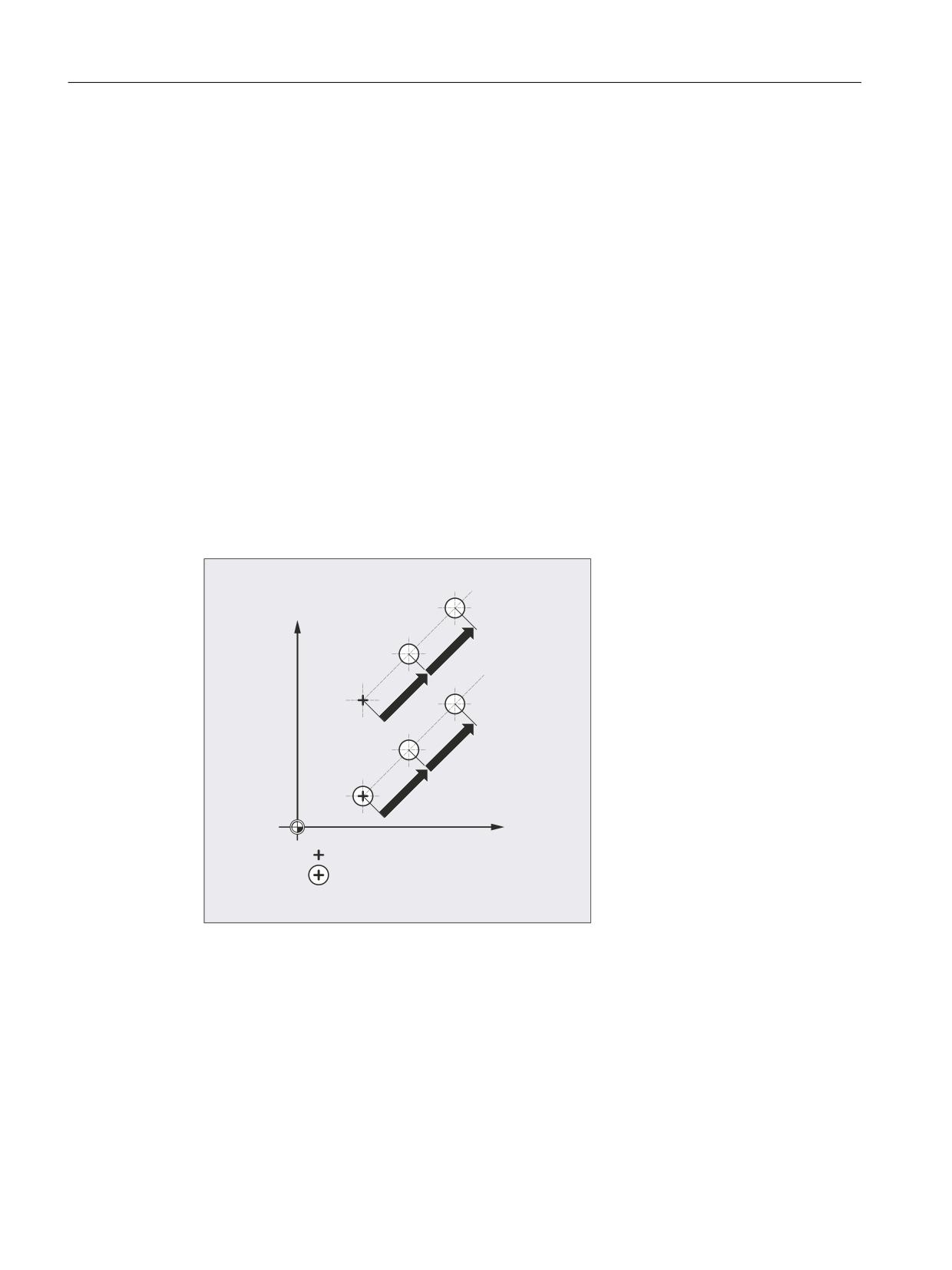
Punching and nibbling
16.1 Activation/deactivation
The axis accelerates at a rate corresponding to 50% of maximum acceleration.
Distance between holes from 2 mm to 10 mm:
Acceleration is increased to 100%, proportional to the spacing.
Distance between holes more than 10 mm:
Traverse at an acceleration of 100%.
Initiation of the first stroke
The instant at which the first stroke is initiated after activation of the function differs depending
on whether nibbling or punching is selected:
● PON/PONS:
- All strokes - even the one in the first block after activation - are executed at the block
end.
● SON/SONS:
- The first stroke after activation of the nibbling function is executed at the start of the
block.
- Each of the following strokes is initiated at the block end.
<
321
621
;
3RVLWLRQ
3RVLWLRQLQJ DQG VWURNH UHOHDVH
Punching and nibbling on the spot
A stroke is initiated only if the block contains traversing information for the punching or nibbling
axes (axes in active plane).
However, to initiate a stroke at the same position, one of the punching/nibbling axes can be
programmed with a traversing path of 0.
Job Planning
614
Programming Manual, 12/2018, A5E40869460B AB

Punching and nibbling
16.1 Activation/deactivation
Machining with rotatable tools
Note
Use the tangential control function if you wish to position rotatable tools at a tangent to the
programmed path.
Use of M commands
As in earlier versions, macro technology allows special M functions to be used instead of
language commands (compatibility). The M functions and equivalent language commands as
used in earlier systems are as follows:
M20, M23
≙ SPOF
M22
≙ SON
M25
≙ PON
M26
≙ PDELAYON
Example for macro file:
Program code
Comment
DEFINE M25 AS PON
; Punching on
DEFINE M125 AS PONS
; Punching with leader on
DEFINE M22 AS SON
; Nibbling on
DEFINE M122 AS SONS
; Nibbling with leader on
DEFINE M26 AS PDELAYON
; Punching with delay on
DEFINE M20 AS SPOF
; Punching, nibbling off
DEFINE M23 AS SPOF
; Punching, nibbling off
Programming example:
Program code
Comment
N100 X100 M20
; Position without punch initiation.
N110 X120 M22
; Activate nibbling, initiate stroke before and af-
ter motion.
N120 X150 Y150 M25
; Activate punching, initiate stroke at end of mo-
tion.
Job Planning
Programming Manual, 12/2018, A5E40869460B AB
615
Punching and nibbling
16.2 Automatic path segmentation
16.2
Automatic path segmentation
Segmentation into path segments
When punching or nibbling is activated, both SPP and SPN segment the total traversing section
programmed for the path axes into a number of path segments with the same length
(equidistant path segmentation). Internally, each path segment corresponds to a block.
Number of strokes
When punching, the first stroke is realized at the end point of the first path segment; but for
nibbling, at the starting point of the first path segment. Therefore the following numbers are
obtained over the complete traversing section:
Punching: Number of strokes = number of path segments
Nibbling: Number of strokes = number of path segments +1
Auxiliary functions
Auxiliary functions are executed in the first of the generated blocks.
Syntax
SPP=
SPN=
Meaning
SPP:
Size of path segment (maximum distance between strokes); modal
SPN:
Number of path segments per block; modally effective
Job Planning
616
Programming Manual, 12/2018, A5E40869460B AB
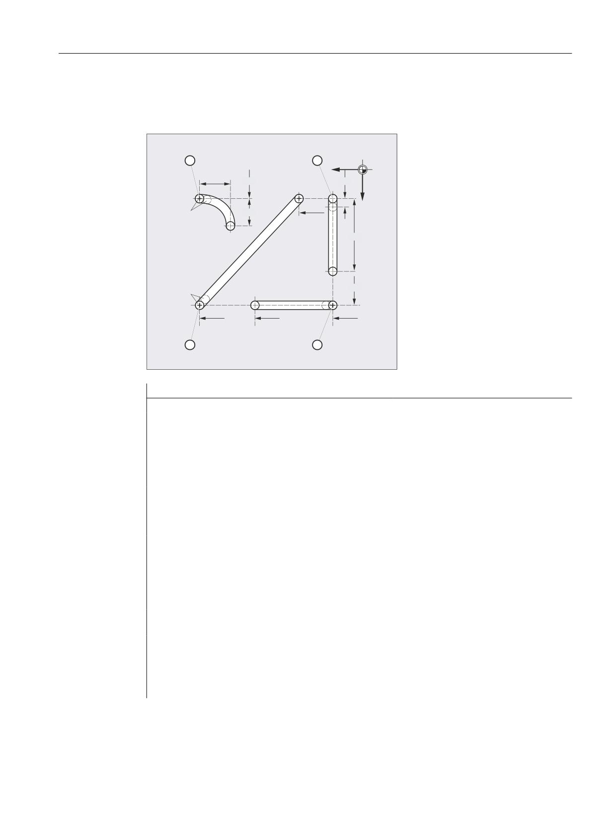
Punching and nibbling
16.2 Automatic path segmentation
Example 1
The programmed nibbling segments should be automatically split-up into path segments.
;
<
Program code
Comment
N100 G90 X130 Y75 F60 SPOF
; Positioning at starting point 1
N110 G91 Y125 SPP=4 SON
; Nibbling on; maximum path seg-
ment length
for automatic path segmentation: 4
mm
N120 G90 Y250 SPOF
; Nibbling off; positioning to
starting point 2
N130 X365 SON
; Nibbling on; maximum path seg-
ment length
for automatic path segmentation: 4
mm
N140 X525 SPOF
; Nibbling off; positioning to
starting point 3
N150 X210 Y75 SPP=3 SON
; Nibbling on; maximum path seg-
ment length
for automatic path segmentation: 3
mm
N160 X525 SPOF
; Nibbling off; positioning to
starting point 4
N170 G02 X-62.5 Y62.5 I J62.5 SPP=3 SON
; Nibbling on; maximum path seg-
ment length
for automatic path segmentation: 3
mm
N180 G00 G90 Y300 SPOF
; Nibbling off
Job Planning
Programming Manual, 12/2018, A5E40869460B AB
617
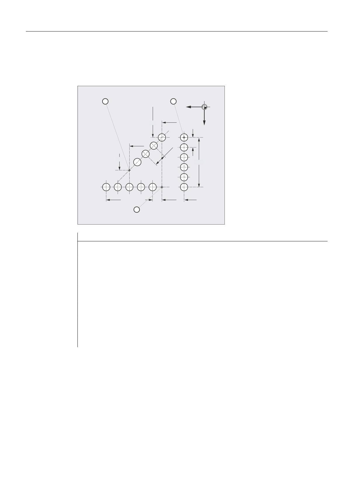
Punching and nibbling
16.2 Automatic path segmentation
Example 2
Automatic path segmentation should be made for the individual series of holes. The maximum
path segment length (SPP value) is specified for the segmentation.
;
<
Program code
Comment
N100 G90 X75 Y75 F60 PON
; Position to starting point 1;
punch a single hole
N110 G91 Y125 SPP=25
; Maximum path segment length for
automatic path segmentation: 25 mm
N120 G90 X150 SPOF
; Punching off; positioning to
starting point 2
N130 X375 SPP=45 PON
; Punching on; maximum path segment length
for automatic path segmentation: 45 mm
N140 X275 Y160 SPOF
; Punching off; positioning to
starting point 3
N150 X150 Y75 SPP=40 PON
; Punching on, instead of the programmed path segment
length of 40 mm, the calculated path segment length of
37.79 mm is used.
N160 G00 Y300 SPOF
; Punching off; positioning
16.2.1
Path segmentation for path axes
Length of SPP path segment
SPP is used to specify the maximum distance between strokes and thus the maximum length
of the path segments in which the total traversing distance is to be divided. The command is
deactivated with SPOF or SPP=0.
Example:
Job Planning
618
Programming Manual, 12/2018, A5E40869460B AB
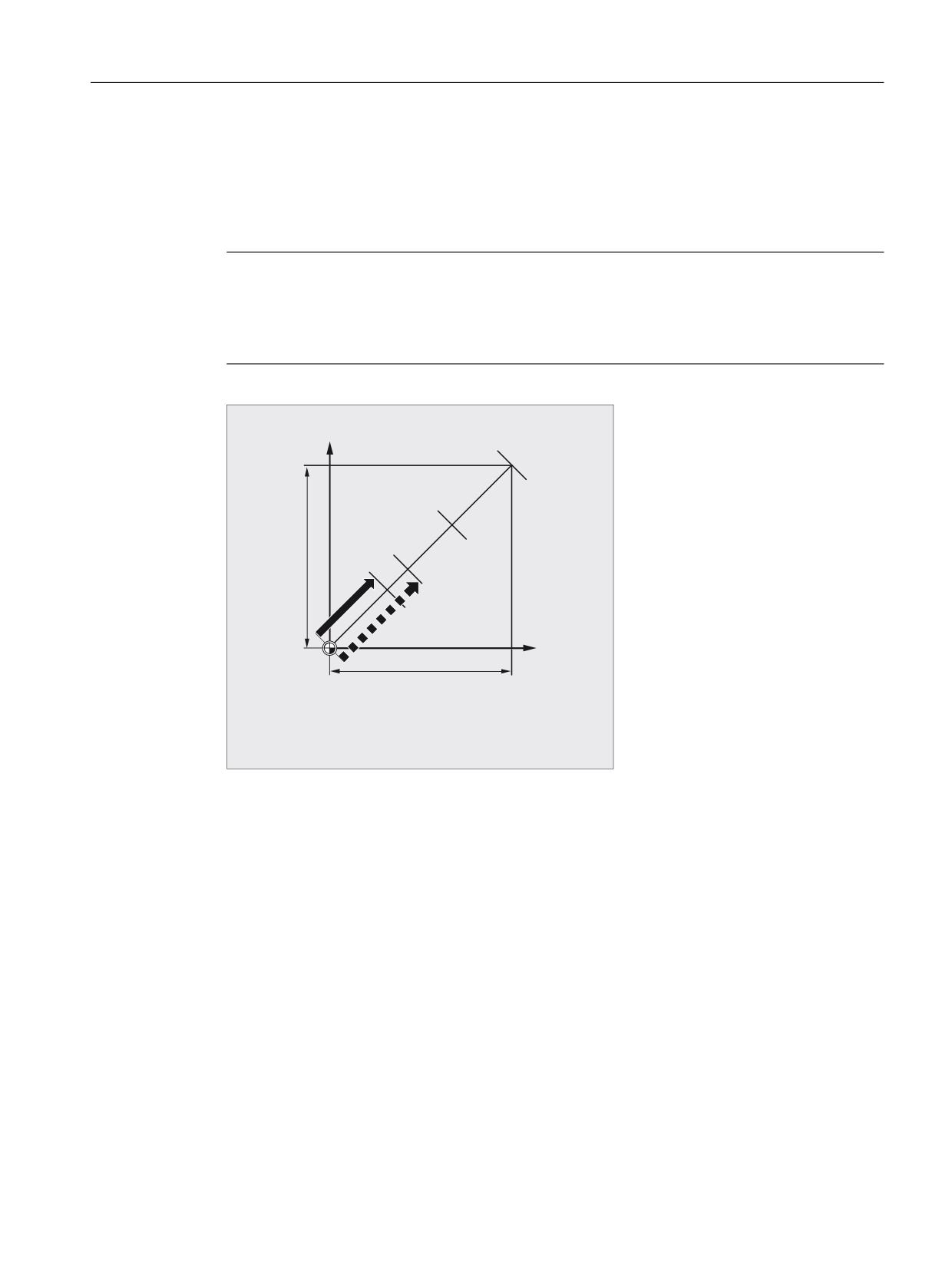
Punching and nibbling
16.2 Automatic path segmentation
N10 SON X0 Y0
N20 SPP=2 X10
The total traversing distance of 10 mm will be divided into five path sections each of 2 mm
(SPP=2).
Note
The path segments effected by SPP are always equidistant, i.e. all segments are equal in
length. In other words, the programmed path segment size (SPP setting) is valid only if the
quotient of the total traversing distance and the SPP value is an integer. If this is not the case,
the size of the path segment is reduced internally such as to produce an integer quotient.
<
<
(
(
;
;
;
< 3URJUDPPHG WUDYHUVH SDWK QLEEOLQJ RU SXQFKLQJ EORFN
(
3URJUDPPHG SDWK VHJPHQW OHQJWK
(
$XWRPDWLFDOO\ URXQGHG SDWK VHJPHQW OHQJWK
Example:
N10 G1 G91 SON X10 Y10
N20 SPP=3.5 X15 Y15
When the total traversing distance is 15 mm and the path segment length 3.5 mm, the quotient
is not an integer value (4.28). In this case, the SPP value is reduced down to the next possible
integer quotient. The result in this example would be a path segment length of 3 mm.
Number of SPN path segments
SPN defines the number of path segments to be generated from the total traversing distance.
The length of the segments is calculated automatically. Since SPN is non-modal, punching or
nibbling must be activated beforehand with PON or SON respectively.
Job Planning
Programming Manual, 12/2018, A5E40869460B AB
619
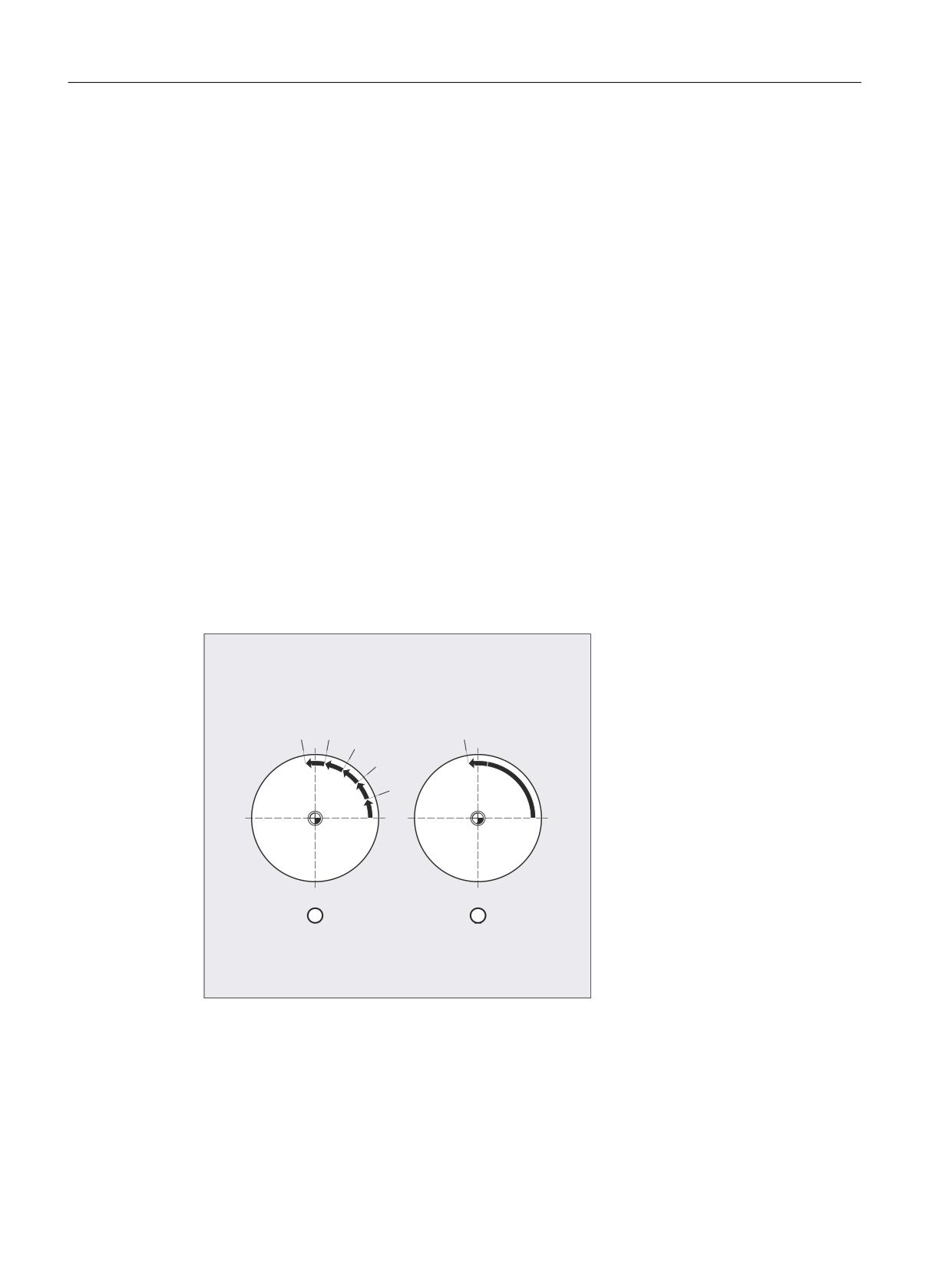
Punching and nibbling
16.2 Automatic path segmentation
16.2.2
Path segmentation for single axes
If single axes are defined as punching/nibbling axes in addition to path axes, then the automatic
path segmentation function can be activated for them.
Behavior of the single axis for SPP
The programmed path segment length (SPP) basically refers to the path axes. Therefore, in a
block in which in addition to the single-axis movement and the SPP value no path axis has
been programmed, then the SPP value is ignored.
If both individual and path axes are programmed in the block, then the behavior of the single
axis depends on the setting of the appropriate machine data.
1. Default setting
The path traversed by the single axis is distributed evenly among the intermediate blocks
generated by SPP.
Example:
N10 G1 SON X10 A0
N20 SPP=3 X25 A100
As a result of the stroke distance of 3 mm, for the total traversing distance of the X axis (path
axis) of 15 mm, 5 blocks are generated.
The A axis thus rotates through 20 degrees in every block.
1. Single axis without path segmentation
The single axis traverses its complete distance in the first of the generated blocks.
2. Different path segmentation
The behavior of the single axis is dependent on the interpolation of the path axes:
Job Planning
620
Programming Manual, 12/2018, A5E40869460B AB
Punching and nibbling
16.2 Automatic path segmentation
● Circular interpolation: Path segmentation
● Linear interpolation: no path segmentation
Behavior for SPN
The programmed number of path segments also applies if a path axis is not simultaneously
programmed.
Precondition: The single axis is defined as punching-nibbling axis.
Job Planning
Programming Manual, 12/2018, A5E40869460B AB
621
Punching and nibbling
16.2 Automatic path segmentation
Job Planning
622
Programming Manual, 12/2018, A5E40869460B AB
Grinding
17
17.1
Activate/deactivate grinding-specific tool monitoring (TMON, TMOF)
With the predefined procedures TMON(...) and TMOF(...), the grinding-specific tool monitoring
is activated or deactivated (geometry and speed monitoring).
Requirement
The tool-specific parameters $TC_TPG1 to $TC_TPG9 must be set.
Syntax
TMON(<TNo>)
TMOF(<TNo>)
Meaning
TMON(...):
Activate grinding-specific tool monitoring
The command must be programmed in the channel in which the grinding-specific tool
monitoring is to be activated.
TMOF(...):
Deactivate grinding-specific tool monitoring
The command must be programmed in the channel in which the grinding-specific tool
monitoring is to be deactivated.
<TNo>:
T number
Note:
Only required if the monitoring is to be switched on or off for an inactive grinding wheel
rather than the active grinding wheel that is currently in use.
TMOF(0):
Deactivate monitoring for all tools
Job Planning
Programming Manual, 12/2018, A5E40869460B AB
623
Grinding
17.1 Activate/deactivate grinding-specific tool monitoring (TMON, TMOF)
Job Planning
624
Programming Manual, 12/2018, A5E40869460B AB

Additional functions
18
18.1
Axis functions (AXNAME, AX, SPI, AXTOSPI, ISAXIS, AXSTRING,
MODAXVAL)
"AXNAME" is used, e.g. to generate cycles that are generally valid, if the names of the axes
are not known.
"AX" is used to indirectly program geometry and synchronous axes. The axis identifier is saved
in a type AXIS variable or is supplied from a command such as "AXNAME" or "SPI".
"SPI" is used if axis functions are programmed for a spindle, e.g. a synchronous spindle.
"AXTOSPI" is used to convert an axis identifier into a spindle index (inverse function to "SPI").
"AXSTRING" is used to convert an axis identifier (data type AXIS) into a string (inverse function
to "AXNAME").
"ISAXIS" is used in universal cycles in order to ensure that a specific geometry axis exists and
thus that any following $P_AXNX call is not aborted with an error message.
"MODAXVAL" is used in order to determine the modulo position for modulo rotary axes.
Syntax
AXNAME("string")
AX[AXNAME("string")]
SPI(n)
AXTOSPI(A) or AXTOSPI(B) or AXTOSPI(C)
AXSTRING( SPI(n) )
ISAXIS(<geometry axis number>)
<Modulo position>=MODAXVAL(<axis>,<axis position>)
Meaning
AXNAME:
Converts an input string into axis identifiers; the input string must contain a valid
axis name.
AX:
Variable axis identifier
SPI:
Converts the spindle number into an axis identifier; the transfer parameter must
contain a valid spindle number.
n:
Spindle number
AXTOSPI:
Converts an axis identifier into an integer spindle index. "AXTOSPI" corresponds
to the inverse function to "SPI".
X, Y, Z:
Axis identifier of AXIS type as variable or constant
AXSTRING:
The string is output with the associated spindle number.
Job Planning
Programming Manual, 12/2018, A5E40869460B AB
625

Additional functions
18.1 Axis functions (AXNAME, AX, SPI, AXTOSPI, ISAXIS, AXSTRING, MODAXVAL)
ISAXIS:
Checks whether the specified geometry axis exists.
MODAXVAL:
For modulo rotary axes, determines the modulo position; this corresponds to
the modulo rest referred to the parameterized modulo range (in the default set-
ting, this is 0 to 360 degrees; the start and size of the modulo range can be
changed using MD30340 MODULO_RANGE_START and MD30330
$MA_MODULO_RANGE).
Note
SPI extensions
The axis function SPI(n) can also be used to read and write frame components. This means
that frames can be written, e.g. with the syntax $P_PFRAME[SPI(1),TR]=2.22.
An axis can be traversed by additionally programming axis positions using the address
AX[SPI(1)]=<axis position>. The prerequisite is that the spindle is either in the
positioning or axis mode.
Examples
Example 1: AXNAME, AX, ISAXIS
Program code
Comment
OVRA[AXNAME("Transverse axis")]=10
; Override for transverse axis
AX[AXNAME("Transverse axis")]=50.2
; End position for transverse axis
OVRA[SPI(1)]=70
; Override for spindle 1
AX[SPI(1)]=180
; End position for spindle 1
IF ISAXIS(1) == FALSE GOTOF CONTINUE
; Abscissa available?
AX[$P_AXN1]=100
; Move abscissa
CONTINUE:
Example 2: AXSTRING
When programming with AXSTRING[SPI(n)], the axis index of the axis, which is assigned to
the spindle, is no longer output as spindle number, but instead the string "Sn" is output.
Program code
Comment
AXSTRING[SPI(2)]
; String "S2" is output.
Example 3: MODAXVAL
The modulo position of modulo rotary axis A is to be determined.
Axis position 372.55 is the starting value for the calculation.
The parameterized modulo range is 0 to 360 degrees:
MD30340 MODULO_RANGE_START = 0
MD30330 $MA_MODULO_RANGE = 360
Program code
Comment
R10=MODAXVAL(A,372.55)
; Calculated modulo position R10 = 12.55.
Job Planning
626
Programming Manual, 12/2018, A5E40869460B AB