SINUMERIK 840D sl/828D. Job Planning. Programming Manual (2010-2018) - page 8

Tool offsets
11.12 Working with tool environments
However, since the wear is evaluated negatively, due to setting data SD42930
$SC_WEAR_SIGN, the compensation determined in this way has to be entered in the
compensation memory with a negative sign. The contents of the relevant tool parameters at
the end of the program are thus:
$TC_DP3[1,1]: 10.000 ; geometry L1 (unchanged)
$TC_DP4[1,1] : 15.000 ; geometry L2 (unchanged)
$TC_DP5[1,1]: 10.000 ; geometry L3 (unchanged)
$TC_DP12[1,1] : 2.010 ; wear L1 (= 10 - 15 * cos(30) + 10 * sin(30))
$TC_DP13[1,1] : -16.160 ; wear L2 (= -15 * sin(30) - 10 * cos(30))
$TC_DP14[1,1] : -5.000 ; wear L3
The effect of setting data SD42930 $SC_WEAR_SIGN on the L3 component in the Y direction
can be recognized without the additional complication caused by the frame rotation.
Additional information
Turning/grinding tools: Calculating the tool length depending on MD20360
$MC_TOOL_PARAMETER_DEF_MASK
The following machine data defines how the wear and tool length are to be evaluated if a
diameter axis is used for turning/grinding tools:
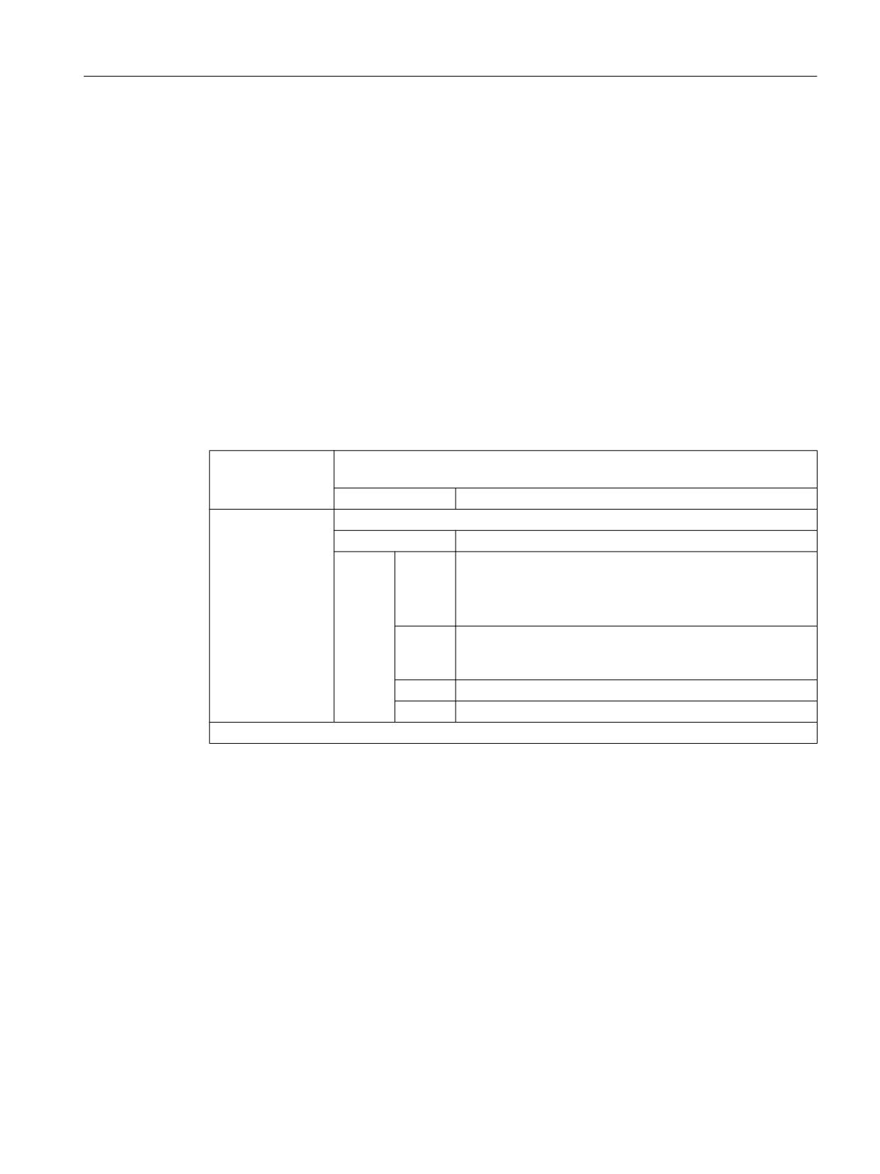
MD20360 $MC_TOOL_PARAMETER_DEF_MASK.<Bit> = <Value>
<Bit>
<Value>
Meaning
0
0
For turning/grinding tools, the wear parameter of the transverse axis is taken into
account in the radius value:
1
For turning/grinding tools, the wear parameter of the transverse axis is taken into
account as the diameter value:
1
0
For turning/grinding tools, the tool length component of the transverse axis is taken
into account as the radius value:
1
For turning/grinding tools, the tool length component of the transverse axis is taken
into account as the diameter value:
If the bits involved are set, the associated entry is weighted with a factor of 0.5. The correction
using SETTCOR is executed so that the total effective tool length change is equal to the value
transferred in <CorVal>. If, when calculating the length, a length is evaluated with a factor of
0.5 as a result of machine data MD20360 $MC_TOOL_PARAMETER_DEF_MASK, then the
compensation of this component must be realized with twice the value transferred.
Example
MD20360 $MC_TOOL_PARAMETER_DEF_MASK = 2 (tool length must be evaluated in the
diameter axis using a factor of 0.5)
Axis X is the diameter axis.
Program code
Comment
N10 DEF REAL _LEN[11]
N20 DEF REAL _CORVAL[3]
N30 $TC_DP1[1,1]=500
; Tool type
Job Planning
Programming Manual, 12/2018, A5E40869460B AB
489
Tool offsets
11.12 Working with tool environments
Program code
Comment
N40 $TC_DP2[1,1]=2
; Cutting edge position
N50 $TC_DP3[1,1]=3.
; Geometry - length 1
N60 $TC_DP4[1,1]=4.
; Geometry - length 2
N70 $TC_DP5[1,1]=5.
; Geometry - length 3
N80 _CORVAL[0]=1.
N90 _CORVAL[1]=1.
N100 _CORVAL[2]=1.
N110 T1 D1 G18 G0 X0 Y0 Z0
; ==> MCS position X1.5 Y5 Z4
N120 R1=SETTCOR(_CORVAL,"G",1,1)
N130 T1 D1 X0 Y0 Z0
; ==> MCS position X2.5 Y6 Z5
N140 R3=$TC_DP3[1,1]
; = 5. = (3.000 + 2.*1.000)
N150 R4=$TC_DP4[1,1]
; = 5. = (4.000 + 1.000)
N160 R5=$TC_DP5[1,1]
; = 6. = (5.000 + 1.000)
N170 M30
In each axis, the tool length compensation should be 1 mm (N80 to N100). 1 mm is thus added
to the original length in lengths L2 and L3. Twice the compensation value (2 mm) is added to
the original tool length in L1, in order to change the total length by 1 mm as required. If the
positions approached in blocks N110 and N130 are compared, it can be seen that each axis
position has changed by 1 mm.
Job Planning
490
Programming Manual, 12/2018, A5E40869460B AB
Tool offsets
11.13 Read the assignment of the tool lengths L1, L2, L3 to the coordinate axes (LENTOAX)
11.13
Read the assignment of the tool lengths L1, L2, L3 to the coordinate
axes (LENTOAX)
The LENTOAX function provides information about the assignment of tool lengths L1, L2 and
L3 of the active tool to the abscissa, ordinate and applicate. The assignment of abscissa,
ordinate and applicate to the geometry axes is affected by frames and the active plane (G17
- G19).
Only the geometry component of a tool ($TC_DP3[<t>,<d>] to $TC_DP5[<t>,<d>]) is
considered, i.e. a different axis assignment for other components (e.g. wear) has no effect on
the result.
Syntax
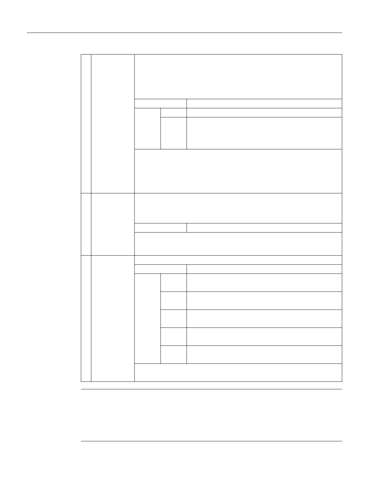
<Status> = LENTOAX(<AxInd>, <Matrix>[, <Coord>])
Principle
LENTOAX(...):
Predefined function to read the assignment of tool lengths L1, L2 and L3 of the
active tool to the coordinate axes
Alone in the block:
Yes
<Status>:
Function return value. Negative values indicate error states.
Data type:
INT
Value:
0
Function OK
Information provided in <AxInd> is sufficient for the descrip-
tion (all tool length components are in parallel to the geom-
etry axes).
1
Function is OK, however, the content of <Matrix> must be
evaluated for a correct description (the tool length compo-
nents are not parallel to the geometry axes).
-1
Invalid string in parameter <Coord>.
-2
No tool active.
Parameters
Job Planning
Programming Manual, 12/2018, A5E40869460B AB
491
Tool offsets
11.13 Read the assignment of the tool lengths L1, L2, L3 to the coordinate axes (LENTOAX)
1
<AxInd>:
If the tool length components are parallel to the geometry axes, the axis indices
assigned to length components L1 to L3 are returned in the <AxInd> array.
● <AxInd> [0]: Abscissa
● <AxInd> [1]: Ordinate
● <AxInd> [2]: Applicate
Data type:
INT[3]
Value:
0
No assignment exists (axis does not exist)
1 ... 3
Number of the length effective in the corresponding coordi-
nate axis.
or
The sign is negative if the tool length component is pointing
-1 ... -3
in the negative coordinate direction.
If not all length components are parallel or antiparallel to the geometry axes, the
index of the axis, which contains the largest part of a tool length component, is
returned in <AxInd>. In this case (if the function does not return an error for a
different reason), then the return value is <Status> = 1. The mapping of tool length
components L1 to L3 to geometry axes 1 to 3 is then described completely by the
content of the 2nd parameter <Matrix>.
2
<Matrix>:
Matrix which represents the vector of the tool lengths (L1=1, L2=1, L3=1) to the
vector of the coordinate axes (abscissa, ordinate, applicate), i.e. the tool length
components are assigned to the columns in the order L1, L2, L3 and the axes are
assigned to the lines in the order abscissa, ordinate, applicate.
Data type:
REAL
All elements are always valid in the matrix, even if the geometry axis belonging
to the coordinate axis is not available, i.e. if the corresponding entry in <AxInd>
is 0.
3
<Coord>:
coordinate system applicable for the assignment (optional)
Data type:
STRING
Charac-
MCS
The tool length is represented in the machine coordinate
ters:
system.
M
BCS
The tool length is represented in the basic coordinate system.
B
WCS
The tool length is represented in the workpiece coordinate
system (default setting).
W
KCS
The tool length is represented in the tool coordinate system
of the kinematic transformation.
K
TCS
The tool length is represented in the tool coordinate system.
T
The notation of the characters in the string (upper or lower case) is arbitrary.
If the parameter <Coord> is not specified, then WCS is used (default setting).
Note
In the TCS, all tool length components are always parallel or antiparallel to the axes.
The components can only be antiparallel when mirroring is active and the following setting
data is activated:
SD42900 $SC_MIRROR_TOOL_LENGTH (sign change tool length when mirroring)
Job Planning
492
Programming Manual, 12/2018, A5E40869460B AB
Tool offsets
11.13 Read the assignment of the tool lengths L1, L2, L3 to the coordinate axes (LENTOAX)
Example
Standard application, milling tool for G17.
L1 applies in Z (applicate), L2 applies in Y (ordinate), L3 applies in X (abscissa).
Function call in the form:
<Status>=LENTOAX(<AxInd>,<Matrix>,"WCS")
The result parameter <AxInd> then contains the values:
<AxInd>[0] = 3
<AxInd>[1] = 2
<AxInd>[2] = 1
Or, in short: (3, 2, 1)
In this case, the associated matrix (<Matrix>) is:
0DWUL[!
A change from G17 to G18 or G19 does not alter the result, because the assignment of the
length components to the geometry axes changes in the same way as the assignment of the
abscissa, ordinate and applicate.
A frame rotation of Z through 60 degrees is now programmed with G17 active, e.g.
ROT Z60
The direction of the applicate (Z direction) remains unchanged; the main component of L2 now
lies in the direction of the new X axis; the main component of L1 now lies in the direction of
the negative Y axis. As a consequence, the return value (<Status>) is "1", <AxInd> contains
the values (2, -3, 1).
In this case, the associated matrix (<Matrix>) is:
VLQ r FRV r
0DWUL[!
FRV r
VLQ r
Job Planning
Programming Manual, 12/2018, A5E40869460B AB
493
Tool offsets
11.13 Read the assignment of the tool lengths L1, L2, L3 to the coordinate axes (LENTOAX)
Job Planning
494
Programming Manual, 12/2018, A5E40869460B AB

Path traversing behavior
12
12.1
Tangential control
12.1.1
Defining coupling (TANG)
Via the predefined procedure TANG(...), a tangential coupling between a rotary axis is defined
as the following axis and two geometry axes as the leading axes. The following axis is
continuously aligned with the path tangent of the leading axes.
Note
Coupling factor
A coupling factor of 1 does not have to be programmed explicitly.
The direction of the tangential axis is rotated using the coupling factor of -1.
Syntax
TANG(<following axis>, <leading axis_1>, <leading axis_2>, <coupling
factor>, <coordinate system>, <optimization>)
Meaning
TANG(...):
Define tangential coupling
<following axis>:
Axis name of the following axis (rotary axis)
Data type:
AXIS
Range of values:
Channel axis names
<leading axis_1>
Axis names of the leading axes (geometry axes) 1)
<leading axis_2>:
Data type:
AXIS
Range of values:
Geometry axis names of the channel
<coupling factor>:
Factor n of the angle change of the following axis for changing the path
tangent of the leading axes:
Angle changefollowing axis = angle changepath tangent * n
Data type:
REAL
Default value:
1.0
<coordinate system>:
Active coordinate system 2)
Data type:
CHAR
Value:
"B":
Basic coordinate system (default value)
"W":
Workpiece coordinate system (not availa-
ble)
Job Planning
Programming Manual, 12/2018, A5E40869460B AB
495

Path traversing behavior
12.1 Tangential control
<optimization>:
Optimization type
Data type:
CHAR
Value:
"S":
Standard (default value)
The dynamic response of the rotary axis
has no effect on the leading axes If the dy-
namic response of the rotary axis is greater
than required for tracking, this method is
sufficiently precise. If the dynamic re-
sponse of the rotary axis is not great
enough to follow the change in the path
tangent, the orientation of the rotary axis
will deviate from the target orientation
along an undefined rounding clearance.
"P":
The dynamic response of the rotary axis is
considered in the path planning of the lead-
ing axes.
For this purpose, on activation of the tan-
gential coupling with TANGON(), two addi-
tional parameters must be specified:
● Rounding clearance
● Angular tolerance
See Section "Activating the coupling (TAN-
GON) (Page 497)"
Note
With kinematic transformations, we recom-
mend using optimization method "P."
Note
Default values do not have to be programmed explicitly.
1) Note
As the leading axes for tangential coupling, the geometry axes must be used that travel along the
programmed path in the machine coordinate system (MCS) with reference to the initial position of the
machine. For example, if swivel cycle CYCLE800 is used on a milling machine with a swivel head,
depending on how the cycle is configured, interpolation will be performed in the WCS, e.g. with the
geometry axes X and Y. The tangential coupling, however, must be defined with the geometry axes as
the leading axes, which travel along the programmed path in the MCS. For this purpose, the geometry
axes in the non-swiveled condition of the machine must be used as the leading axes.
2) Note
The basic coordinate system (BCS) must not be rotated with respect to the MCS. For example, if the
BCS is rotated with the ROT command or with the swivel cycle CYCLE800, the tangential control is no
longer correct.
12.1.2
Activating intermediate block generation (TLIFT)
If the tangent change of the following axis at any position along the programmed path of the
leading axes exceeds the limit parameterized in machine data MD37400
$MA_EPS_TLIFT_TANG_STEP, further path planning will depend on the set behavior at
corners. Without use of the predefined procedure TLIFT(...), the path is traversed in
accordance with the rounding behavior programmed in connection with TANG(...) (Page 495)
and TANGON(...) (Page 497).
Job Planning
496
Programming Manual, 12/2018, A5E40869460B AB
Path traversing behavior
12.1 Tangential control
Activating intermediate block generation
If TLIFT(...) is programmed after TANG(...), an intermediate block automatically generated by
the control is inserted at this point when a corner is detected during preprocessing.
When the program is executed, the leading axes are stopped when the intermediate block is
reached. In the intermediate block, the following axis is rotated with maximum axis dynamics
toward the path tangent of the following block. The leading axes are then traversed further on
the programmed path.
Deactivating intermediate block generation
To deactivate intermediate block generation, the tangential coupling must be defined again
using TANG(...), but without subsequent activation of intermediate block generation by means
of TLIFT(...).
Syntax
TLIFT(<following axis>)
Meaning
TLIFT(...):
Activate corner detection with intermediate block calculation
<following axis>:
Axis name of the following axis (rotary axis)
Data type:
AXIS
Range of values:
Channel axis names
Speed of rotation of the following axis
Path axis
If the following axis had already been traversed as a path axis before tangential coupling was
activated, the rotational movement is performed in the intermediate block as a path axis.
If you specify the reference radius with FGREF[<axis>]=0.001, the rotational movement
will be performed with the parameterized maximum axis velocity:
MD32000 $MA_MAX_AX_VELO[<following axis>]
Positioning axis
If the following axis had not yet been traversed as a path axis before tangential coupling was
activated, the rotation is performed in the intermediate block as a positioning axis.
The rotational movement is performed with the parameterized positioning axis velocity:
MD32060 $MA_POS_AX_VELO[<following axis>]
12.1.3
Activating the coupling (TANGON)
Via the predefined procedure TANGON(...), a tangential coupling previously defined with
TANG(...) (Page 495) is activated. The following axis is then continuously aligned with the path
tangent during subsequent travel.
Job Planning
Programming Manual, 12/2018, A5E40869460B AB
497

Path traversing behavior
12.1 Tangential control
Angle of the following axis
The angle of the following axis with respect to the path tangent depends on the transformation
ratio specified in TANG(...), the offset angle parameterized in the machine data MD37402
$MA_TANG_OFFSET, and the offset angle specified for TANGON(...), which is applied
additively.
Optimization "P"
If the value "P" was specified as the optimization parameter in the definition of the tangential
coupling (TANG(...)), the parameter "rounding clearance" and optionally the parameter
"angular tolerance" must be set when coupling is activated.
If the value 0 is specified as the angular tolerance, only the parameter "rounding clearance"
will be active.
If a value greater than 0 is specified as the angular tolerance, the active rounding clearance
results from the minimum of the parameterized rounding clearance and the rounding clearance
based on the parameterized angular tolerance.
If the dynamic response of the following axis is not sufficient to follow the parameterized
conditions, the path velocity of the leading axes will be reduced accordingly.
Syntax
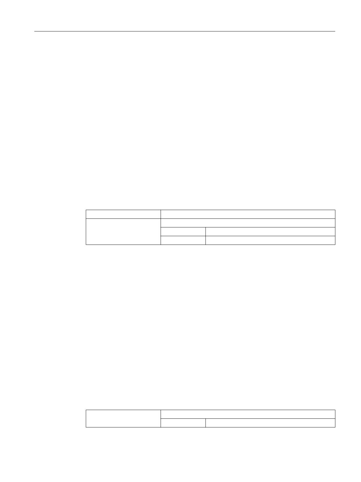
TANGON(<following axis>, <offset angle>, <rounding clearance>,
<angular tolerance>)
Meaning
TANGON(...):
Activate tangential coupling
<following axis>:
Axis name of the following axis (rotary axis)
Data type:
AXIS
Range of values:
Channel axis names
<offset angle>:
Offset angle of following axis with respect to the path tangent
The reference point is the zero point of the rotary axis.
Data type:
REAL
<rounding clearance>:
Maximum permissible rounding clearance
If the rounding clearance is increased due to the dynamic conditions,
the path velocity of the leading axes is reduced.
Data type:
REAL
<angular tolerance>:
Maximum permissible tolerance with respect to the specified angle be-
tween the following axis zero setting and the path tangent
Data type:
REAL
Job Planning
498
Programming Manual, 12/2018, A5E40869460B AB
Path traversing behavior
12.1 Tangential control
12.1.4
Deactivating the coupling (TANGOF)
Via the predefined procedure TANGOF(...), a tangential coupling defined with TANG(...)
(Page 495) and activated with TANGON(...) (Page 497) is deactivated. The following axis is
then no longer aligned with the path tangent of the leading axis. However, the coupling of the
following axis to the leading axes is retained even after deactivation, which prevents the
following functions, for example:
● Plane change
● Geometry axis switchover
● Definition of a new tangential coupling for the following axis
Final cancellation of the connection of the coupling of the following axis to the leading axes is
not completed until the coupling has been deleted with TANGDEL(...) (Page 499).
Programming
TANGOF(<following axis>)
Meaning
TANGOF(...):
Deactivate a tangential coupling
<following axis>:
Axis name of the following axis (rotary axis)
Data type:
AXIS
Range of values:
Channel axis names
12.1.5
Deleting a coupling (TANGDEL)
A tangential coupling defined with TANG(...) (Page 495) will be retained even after deactivation
of the tangential coupling with TANGOF(...) (Page 499). The existing tangential coupling then
continues to prevent, for example, the following functions:
● Plane change
● Geometry axis switchover
● Definition of a new tangential coupling for the following axis
With the predefined procedure TANGDEL(...), the existing tangential coupling is deleted after
the tangential coupling has been deactivated with TANGOF(...).
Syntax
TANGDEL(<following axis>)
Meaning
TANGDEL(...):
Delete a tangential coupling defined with TANG()
Effective:
Non-modal
Job Planning
Programming Manual, 12/2018, A5E40869460B AB
499
Path traversing behavior
12.1 Tangential control
<following axis>:
Axis name of the following axis whose tangential coupling is to be de-
leted
Data type:
AXIS
Range of values:
Channel axis names
Examples
Leading axis change
Before a new tangential coupling can be defined with another leading axis for the following
axis, the existing tangential coupling must first be deleted.
Program code
Comment
N10 TANG(A, X, Y, 1)
; Define tangential couping for following axis A: A to
X and Y
N20 TANGON(A)
; Activate tangential coupling for following axis A
N30 X10 Y20
N80 TANGOF(A)
; Deactivate tangential coupling for following axis A
N90 TANGDEL(A)
; Delete tangential coupling for following axis A
N120 TANG(A, X, Z)
; Define new tangential coupling for following axis A
N130 TANGON(A)
; Activate new tangential coupling for following axis A
Geometry axis switchover
Before geometry axis switchover can be performed for an existing coupling, the coupling must
first be deleted.
Program code
Comment
N10 GEOAX(2,Y1)
; 2nd geometry axis = machine axis Y1
N20 TANG(A, X, Y)
; Define tangential coupling for following axis A
N30 TANGON(A, 90)
; Activate tangential coupling for following axis A
N40 G2 F8000 X0 Y0 I0 J50
; Motion block
N50 TANGOF(A)
; Deactivate tangential coupling for following axis A
N60 TANGDEL(A)
; Delete tangential coupling for following axis A
N70 GEOAX(2, Y2)
; 2nd geometry axis = machine axis Y2
N80 TANG(A, X, Y)
; Define new tangential coupling for following axis A
N90 TANGON(A, 90)
; Activate new tangential coupling for following axis
A
Job Planning
500
Programming Manual, 12/2018, A5E40869460B AB
Path traversing behavior
12.2 Feedrate characteristic (FNORM, FLIN, FCUB, FPO)
12.2
Feedrate characteristic (FNORM, FLIN, FCUB, FPO)
To permit flexible definition of the feedrate characteristic, the feedrate programming according
to DIN 66025 has been extended by linear and cubic characteristics.
The cubic characteristics can be programmed either directly or as interpolating splines. These
additional characteristics make it possible to program continuously smooth velocity
characteristics depending on the curvature of the workpiece to be machined.
These additional characteristics make it possible to program continuously smooth velocity
characteristics depending on the curvature of the workpiece to be machined.
Syntax
F… FNORM
F… FLIN
F… FCUB
F=FPO(…,…,…)
Meaning
FNORM:
Basic setting. The feed value is specified as a function of the traverse path of the block
and is then valid as a modal value.
FLIN:
Path velocity profile linear:
The feed value is approached linearly via the traverse path from the current value at
the block beginning to the block end and is then valid as a modal value. The response
can be combined with G93 and G94.
FCUB:
Path velocity profile cubic:
The blockwise programmed F values (relative to the end of the block) are connected
by a spline. The spline begins and ends tangentially with the previous and following
defined feedrate and takes effect with G93 and G94.
If the F address is missing from a block, the last F value to be programmed is used.
F=FPO… :
Polynomial path velocity profile:
The F address defines the feed characteristic via a polynomial from the current value
to the block end. The end value is valid thereafter as a modal value.
Feed optimization on curved path sections
Feed polynomial F=FPO and feed spline FCUB should always be traversed at constant
cutting rate CFC, thereby allowing a jerk-free setpoint feed profile to be generated. This
enables creation of a continuous acceleration setpoint feed profile.
Job Planning
Programming Manual, 12/2018, A5E40869460B AB
501
Path traversing behavior
12.2 Feedrate characteristic (FNORM, FLIN, FCUB, FPO)
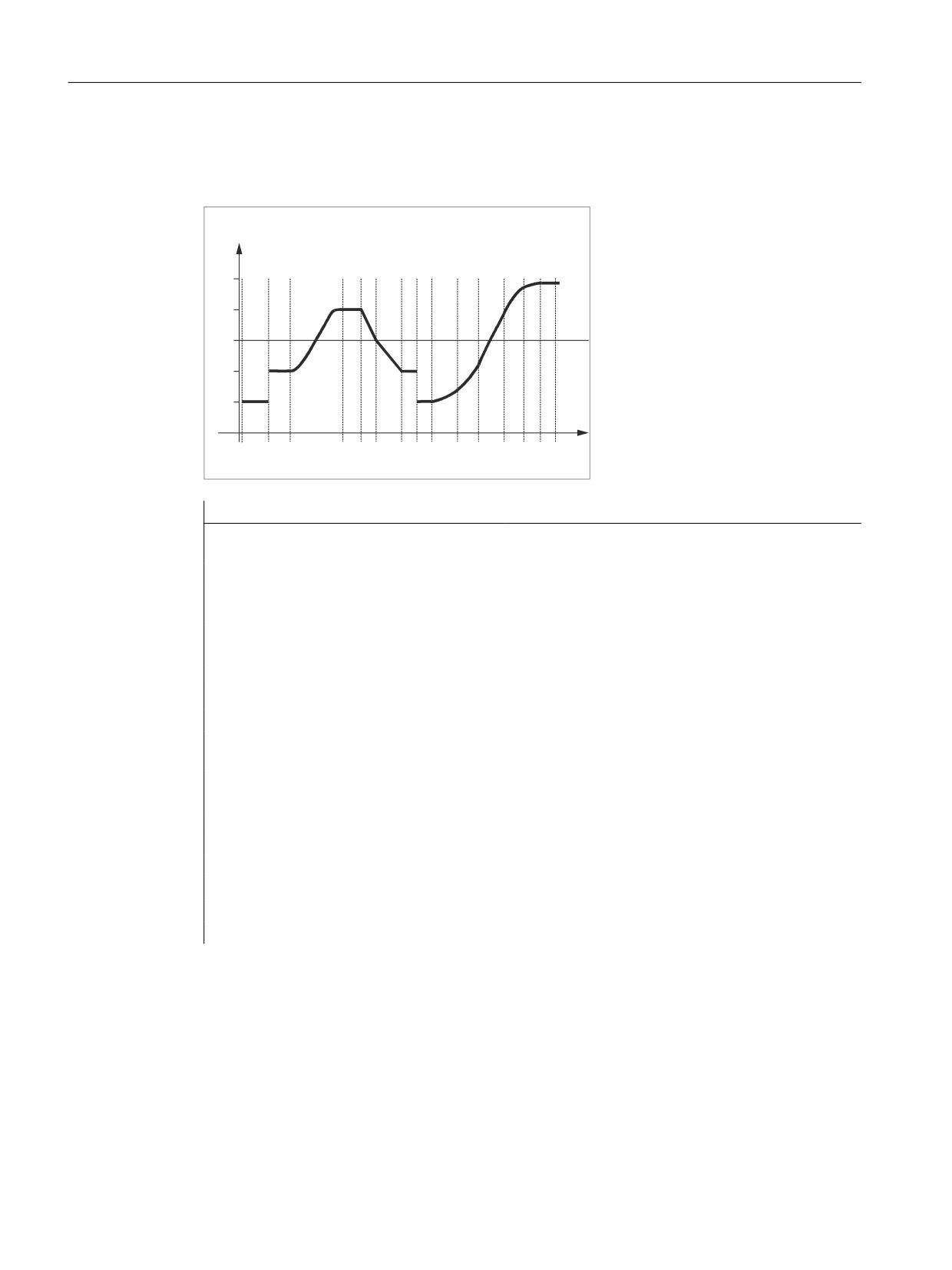
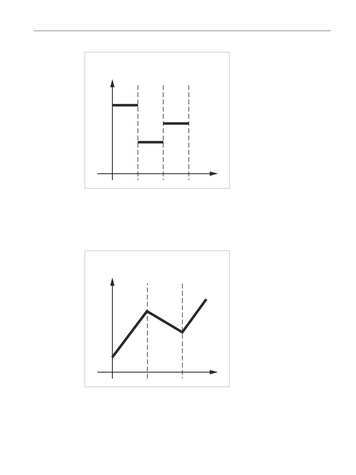
Example: Various feed profiles
This example shows you the programming and graphic representation of various feed profiles.
)HHG
3DWK
1
1
1
1 1
1
1 1
1
1
1
1
1 1 1
Program code
Comment
N1 F1000 FNORM G1 X8 G91 G64
; Constant feedrate profile, incremental di-
mension data
N2 F2000 X7
; Setpoint velocity step change
N3 F=FPO(4000, 6000, -4000)
; Feed profile via polynomial with feed 4000
at the end of the block
N4 X6
; Polynomial feedrate 4000 is valid as modal
value
N5 F3000 FLIN X5
; Linear feedrate profile
N6 F2000 X8
; Linear feedrate profile
N7 X5
; Linear feedrate is valid as modal value
N8 F1000 FNORM X5
; Constant feedrate profile with acceleration
step change
N9 F1400 FCUB X8
; All of the following F values programmed in
blocks are connected with splines
N10 F2200 X6
N11 F3900 X7
N12 F4600 X7
N13 F4900 X5
; Switch-out spline profile
N14 FNORM X5
N15 X20
Further information
FNORM
The feed address F defines the path feedrate as a constant value according to DIN 66025.
Please refer to Programming Manual "Fundamentals" for more detailed information on this
subject.
Job Planning
502
Programming Manual, 12/2018, A5E40869460B AB
Path traversing behavior
12.2 Feedrate characteristic (FNORM, FLIN, FCUB, FPO)
)HHG
3DWK
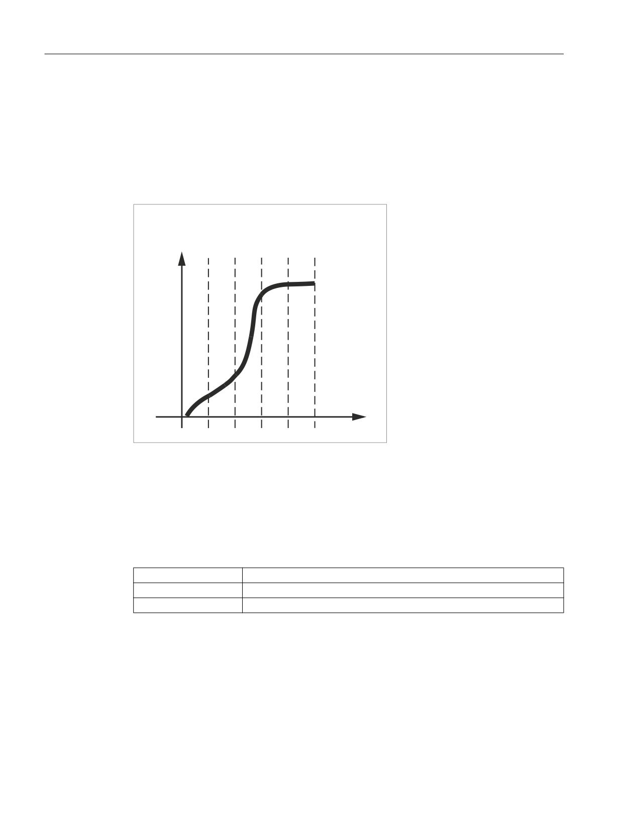
FLIN
The feedrate characteristic is approached linearly from the current feedrate value to the
programmed F value until the end of the block.
Example:
N30 F1400 FLIN X50
)HHG
3DWK
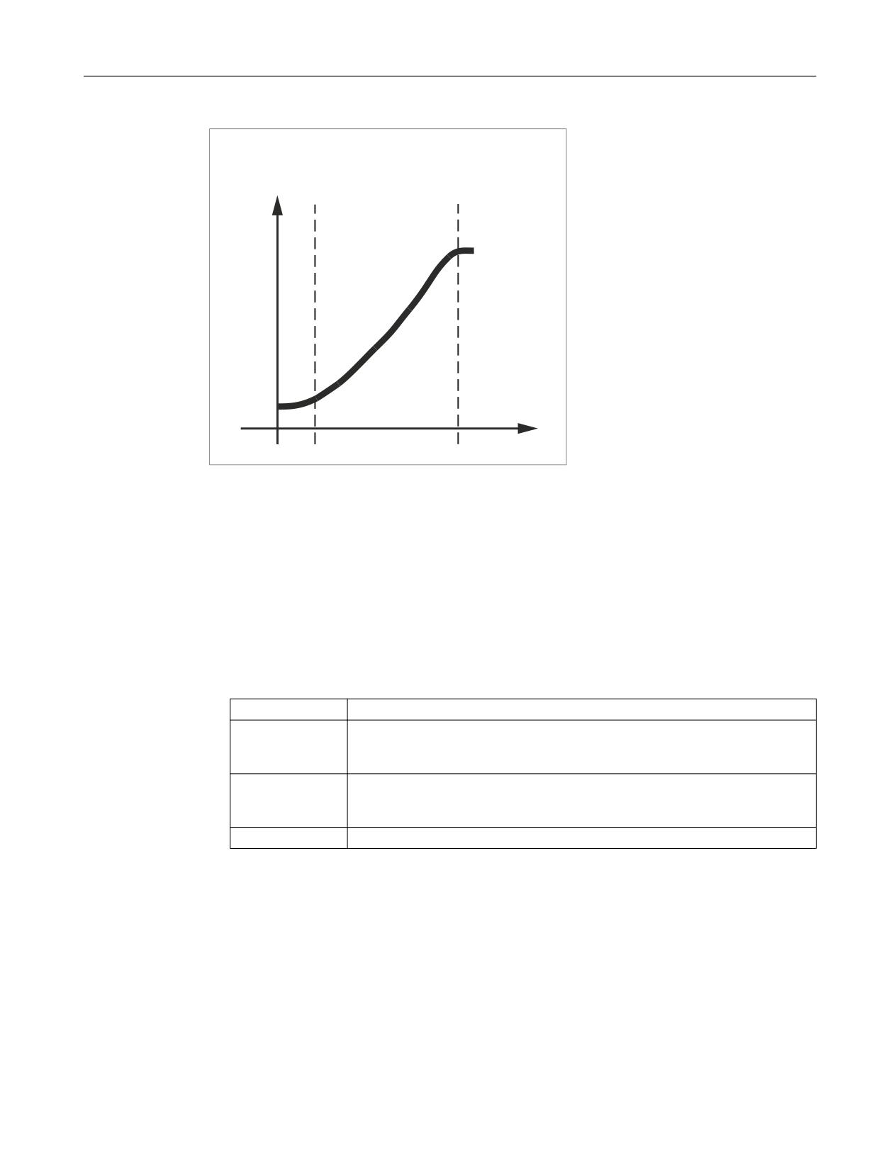
FCUB
The feedrate is approached according to a cubic characteristic from the current feedrate value
to the programmed F value until the end of the block. The control uses splines to connect all
Job Planning
Programming Manual, 12/2018, A5E40869460B AB
503
Path traversing behavior
12.2 Feedrate characteristic (FNORM, FLIN, FCUB, FPO)
the feedrate values programmed non-modally that have an active FCUB. The feedrate values
act here as interpolation points for calculation of the spline interpolation.
Example:
N50 F1400 FCUB X50
N60 F2000 X47
N70 F3800 X52
)HHG
3DWK
F=FPO(…,…,…)
The feedrate characteristic is programmed directly via a polynomial. The polynomial
coefficients are specified according to the same method used for polynomial interpolation.
Example:
F=FPO(endfeed, quadf, cubf)
endfeed, quadf and cubf are previously defined variables.
endfeed:
Feedrate at block end
quadf:
Quadratic polynomial coefficient
cubf:
Cubic polynomial coefficient
With an active FCUB, the spline is linked tangentially to the characteristic defined via FPO at
the block beginning and block end.
Job Planning
504
Programming Manual, 12/2018, A5E40869460B AB
Path traversing behavior
12.2 Feedrate characteristic (FNORM, FLIN, FCUB, FPO)
)HHG
3DWK
Supplementary conditions
● The functions for programming the path traversing characteristics apply regardless of the
programmed feedrate characteristic.
● The programmed feedrate characteristic is always absolute regardless of G90 or G91.
● The feed characteristic curve FLIN and FCUB does not act with G93 and G94 for G95,
G96/G961 and G97/G971.
● With an active compressor COMPON the following applies when several blocks are joined
to form a spline segment:
FNORM:
The F word of the last block in the group applies to the spline segment.
FLIN:
The F word of the last block in the group applies to the spline segment.
The programmed F value applies until the end of the segment and is then
approached linearly.
FCUB:
The generated feedrate spline deviates from the programmed end points by an
amount not exceeding the value set in machine data MD20172 $MC_COM-
PRESS_VELO_TOL.
F=FPO(…,…,…):
These blocks are not compressed.
Job Planning
Programming Manual, 12/2018, A5E40869460B AB
505
Path traversing behavior
12.3 Acceleration behavior
12.3
Acceleration behavior
12.3.1
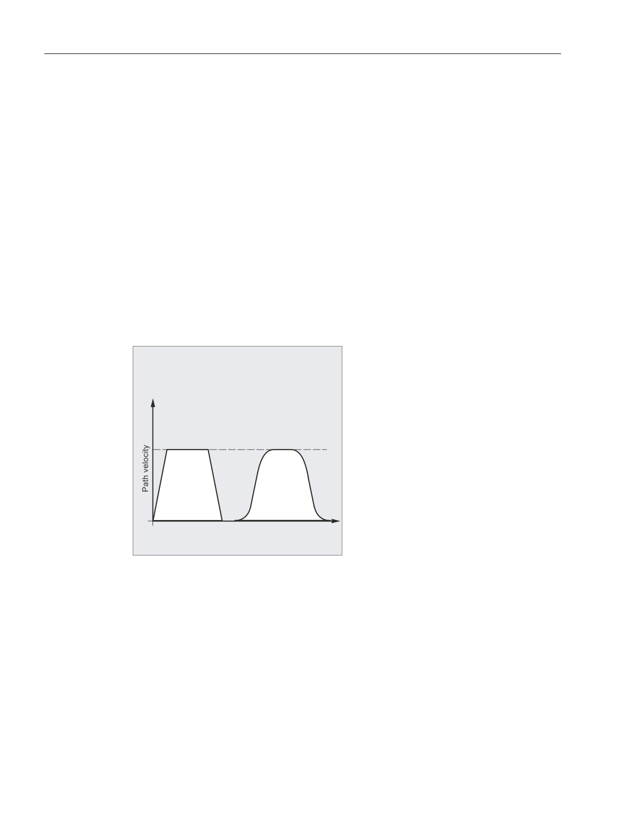
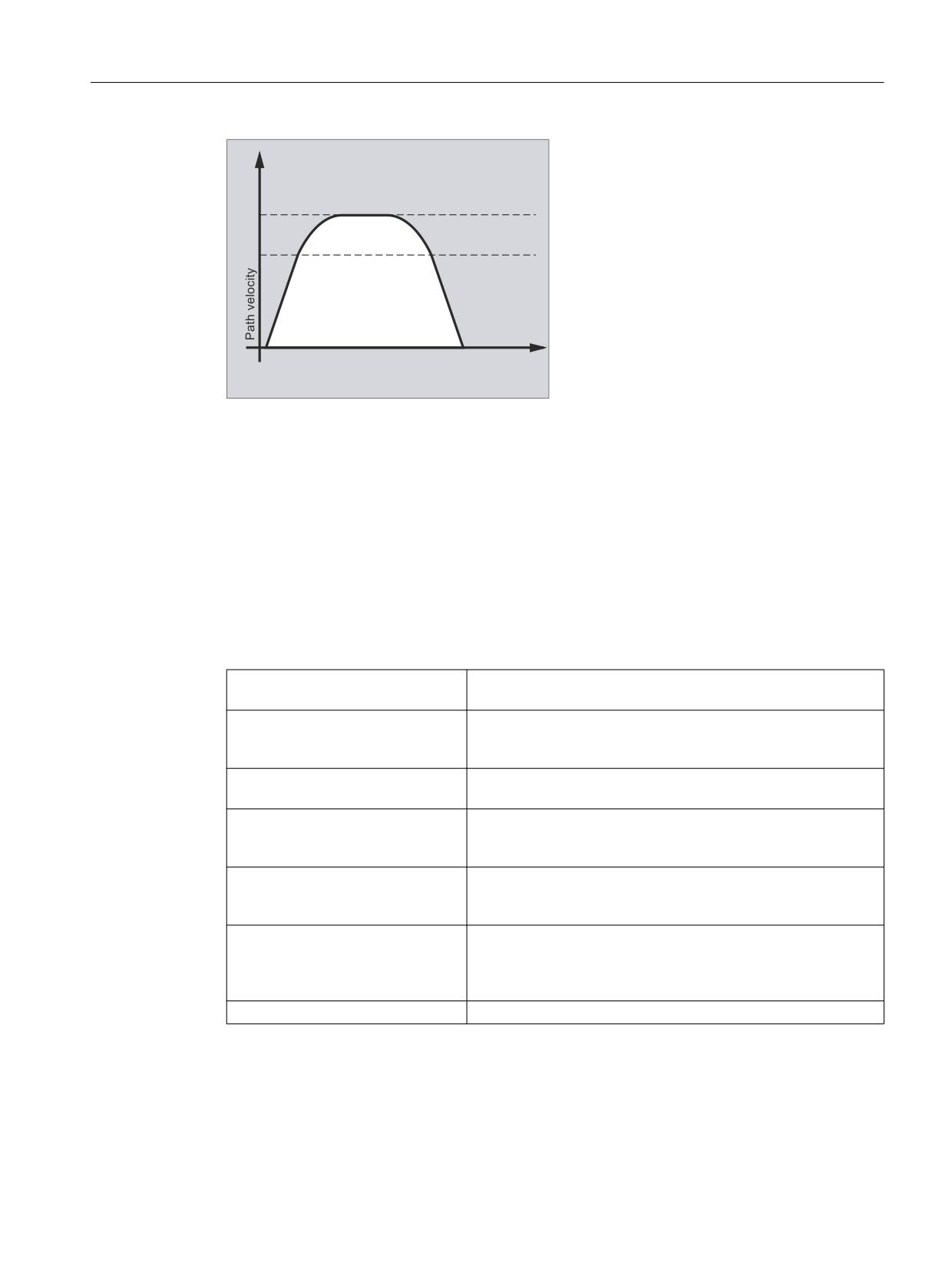
Acceleration mode (BRISK, BRISKA, SOFT, SOFTA, DRIVE, DRIVEA)
The following part program commands are available for programming the current acceleration
mode:
● "BRISK, BRISKA"
The single axes or the path axes traverse with maximum acceleration until the programmed
feedrate is reached (acceleration without jerk limitation).
● "SOFT, SOFTA"
The single axes or the path axes traverse with constant acceleration until the programmed
feedrate is reached (acceleration with jerk limitation).
● "DRIVE, DRIVEA"
The single axes or the path axes traverse with maximum acceleration up to a programmed
velocity limit (MD setting!). The acceleration rate is then reduced (MD setting) until the
programmed feedrate is reached.
6HWSRLQW
%5,6.
62)7
WLPH
SURWHFWLQJ WKH
RSWLPL]HG
PHFKDQLFDO
V\VWHP
7LPH
Figure 12-1
Path velocity curve with BRISK and SOFT
Job Planning
506
Programming Manual, 12/2018, A5E40869460B AB
Path traversing behavior
12.3 Acceleration behavior
6HWSRLQW
/LPLW RI
FRQVWDQW
DFFHOHUDWLRQ
7LPH
Figure 12-2
Path velocity curve with DRIVE
Syntax
BRISK
BRISKA(<axis1>,<axis2>,…)
SOFT
SOFTA(<axis1>,<axis2>,…)
DRIVE
DRIVEA(<axis1>,<axis2>,…)
Meaning
BRISK:
Command for activating the "acceleration without jerk limitation"
for the path axes.
BRISKA:
Command for activating the "acceleration without jerk limitation"
for single axis movements (JOG, JOG/INC, positioning axis, os-
cillating axis, etc.).
SOFT:
Command for activating the "acceleration with jerk limitation" for
the path axes.
SOFTA:
Command for activating the "acceleration with jerk limitation" for
single axis movements (JOG, JOG/INC, positioning axis, oscil-
lating axis, etc.).
DRIVE:
Command for activating the reduced acceleration above a con-
figured velocity limit (MD35220 $MA_ACCEL_REDUC-
TION_SPEED_POINT) for the path axes.
DRIVEA:
Command for activating the reduced acceleration above a con-
figured velocity limit (MD35220 $MA_ACCEL_REDUC-
TION_SPEED_POINT) for single axis movements (JOG, JOG/
INC, positioning axis, oscillating axis, etc.).
(<axis1>,<axis2>, etc.):
Single axes for which the called acceleration mode is to apply.
Job Planning
Programming Manual, 12/2018, A5E40869460B AB
507
Path traversing behavior
12.3 Acceleration behavior
Supplementary conditions
Changing acceleration mode during machining
If the acceleration mode is changed in a part program during machining (BRISK ↔ SOFT), then
there is a block change with exact stop at the end of the block during the transition even with
continuous-path mode.
Examples
Example 1: SOFT and BRISKA
Program code
N10 G1 X… Y… F900 SOFT
N20 BRISKA(AX5,AX6)
Example 2: DRIVE and DRIVEA
Program code
N05 DRIVE
N10 G1 X… Y… F1000
N20 DRIVEA (AX4, AX6)
References
Function Manual, Basic Functions; Acceleration (B2)
12.3.2
Influence of acceleration on following axes (VELOLIMA, ACCLIMA, JERKLIMA)
In the case of axis couplings (tangential correction, coupled motion, master value coupling,
electronic gear; see "Axis couplings (Page 541)").
The dynamics limits of the following axes/spindles can be manipulated using the VELOLIMA,
ACCLIMA, and JERKLIMA functions from the part program or from synchronized actions, even
if the axis coupling is already active.
Note
The JERKLIMA function is not available for all types of coupling.
References:
● Function Manual, Special Functions; Axis Couplings (M3)
● Function Manual, Extended Functions; Synchronous Spindle (S3)
Job Planning
508
Programming Manual, 12/2018, A5E40869460B AB

Path traversing behavior
12.3 Acceleration behavior
Note
Availability for SINUMERIK 828D
The VELOLIMA, ACCLIMA and JERKLIMA functions can only be used with SINUMERIK 828D
in conjunction with the "coupled motion" function!
Syntax
VELOLIMA(<axis>)=<value>
ACCLIMA(<axis>)=<value>
JERKLIMA(<axis>)=<value>
Meaning
VELOLIMA:
Command to correct the parameterized maximum velocity
ACCLIMA:
Command to correct the parameterized maximum acceleration
JERKLIMA:
Command to correct the parameterized maximum jerk
<axis>:
Following axis whose dynamics limits need to be corrected
<value>:
Percentage correction value
Examples
Example 1: Correction of the dynamics limits for a following axis (AX4)
Program code
Comment
VELOLIMA[AX4]=75
; Limit correction to 75% of the maximum axial velocity
stored in the machine data
ACCLIMA[AX4]=50
; Limit correction to 50% of the maximum axial acceleration
stored in the machine data
JERKLIMA[AX4]=50
; Limit correction to 50% of the maximum axial jerk stored
in the machine data
Example 2: Electronic gear
Axis 4 is coupled to axis X via an "electronic gear" coupling. The acceleration capacity of the
following axis is limited to 70% of the maximum acceleration. The maximum permissible
velocity is limited to 50% of the maximum velocity. Once the coupling has been activated
successfully, the maximum permissible velocity is restored to 100%.
Program code
Comment
N120 ACCLIMA[AX4]=70
; Reduced maximum acceleration.
N130 VELOLIMA[AX4]=50
; Reduced maximum velocity.
N150 EGON(AX4,"FINE",X,1,2)
; Activation of the EG coupling.
Job Planning
Programming Manual, 12/2018, A5E40869460B AB
509
Path traversing behavior
12.3 Acceleration behavior
Program code
Comment
N200 VELOLIMA[AX4]=100
; Full maximum velocity.
Example 3: Influencing master value coupling by static synchronized action
Axis 4 is coupled to X by master value coupling. The acceleration response is limited to position
80% by static synchronized action 2 from position 100.
Program code
Comment
N120 IDS=2 WHENEVER $AA_IM[AX4] >
; Synchronized action
100 DO ACCLIMA[AX4]=80
N130 LEADON(AX4, X, 2)
; Master value coupling on
12.3.3
Activation of technology-specific dynamic values (DYNNORM, DYNPOS,
DYNROUGH, DYNSEMIFIN, DYNFINISH)
Using the "Technology" G group, the appropriate dynamic response can be activated for five
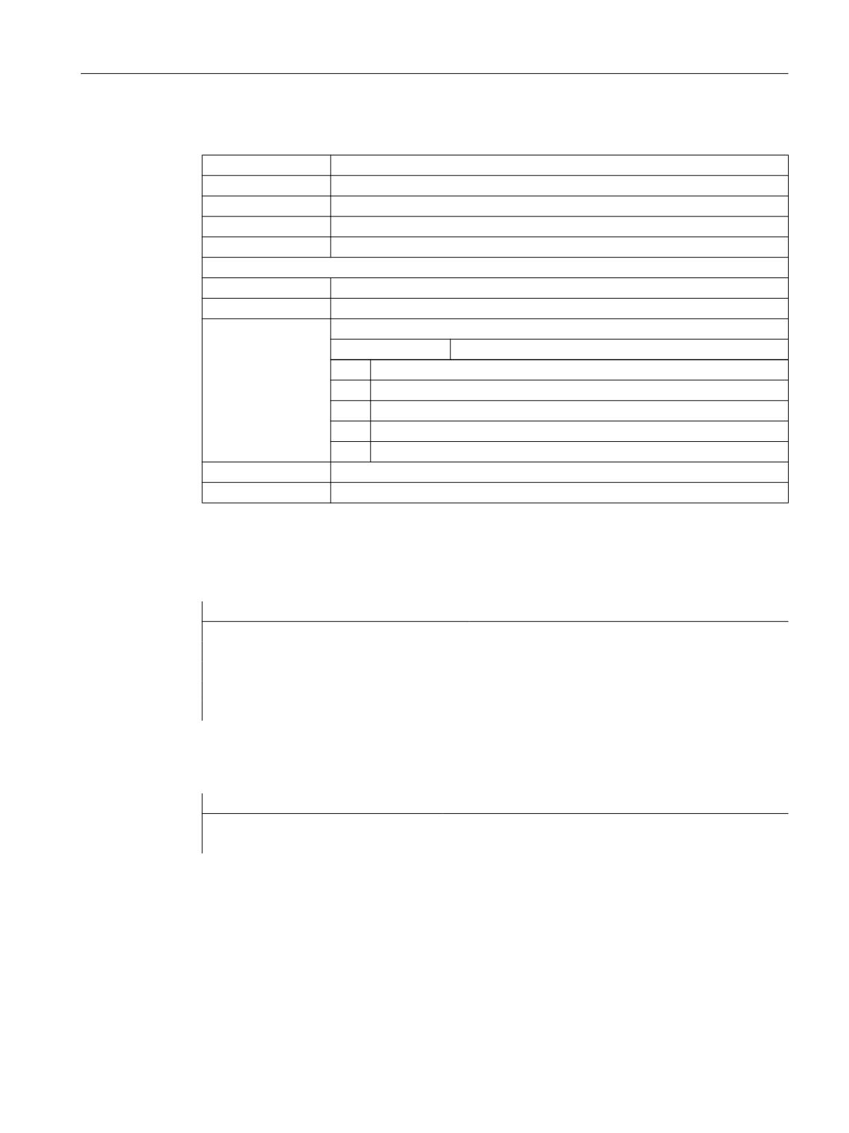
varying technological machining steps.
Dynamic values and G commands can be configured and are, therefore, dependent on
machine data settings (→ machine manufacturer).
References:
Function Manual, Basic Functions; Continuous-Path Mode, Exact Stop, Look Ahead (B1)
Syntax
Activate dynamic values:
DYNNORM
DYNPOS
DYNROUGH
DYNSEMIFIN
DYNFINISH
Note
The dynamic values are already active in the block in which the associated G command is
programmed. Machining is not stopped.
Read or write a specific field element:
R<m>=$MA...[n,X]
$MA...[n,X]=<value>
Job Planning
510
Programming Manual, 12/2018, A5E40869460B AB
Path traversing behavior
12.3 Acceleration behavior
Meaning
DYNNORM:
G command for activating the normal dynamic response
DYNPOS:
G command for activating the dynamic response for positioning mode, tapping
DYNROUGH:
G command for activating the dynamic response for roughing
DYNSEMIFIN:
G command for activating the dynamic response for finishing
DYNFINISH:
G command for activating the dynamic response for smooth-finishing
R<m>:
R-parameter with number <m>
$MA...[n,X]:
Machine data with field element affecting dynamic response
<n>:
Array index
Range of values:
0 ... 4
0
Normal dynamic response (DYNNORM)
1
Dynamic response for positioning mode (DYNPOS)
2
Dynamic response for roughing (DYNROUGH)
3
Dynamic response for finishing (DYNSEMIFIN)
4
Dynamic response for smooth-finishing (DYNFINISH)
<X> :
Axis address
<value>:
Dynamic value
Examples
Example 1: Activate dynamic values
Program code
Comment
DYNNORM G1 X10
; Initial setting
DYNPOS G1 X10 Y20 Z30 F…
; Positioning mode, tapping
DYNROUGH G1 X10 Y20 Z30 F10000
;Roughing
DYNSEMIFIN G1 X10 Y20 Z30 F2000
;Finishing
DYNFINISH G1 X10 Y20 Z30 F1000
; Smooth finishing
Example 2: Read or write a specific field element
Maximum acceleration for roughing, axis X
Program code
Comment
R1=$MA_MAX_AX_ACCEL[2,X]
; reading
$MA_MAX_AX_ACCEL[2,X]=5
; writing
Job Planning
Programming Manual, 12/2018, A5E40869460B AB
511
Path traversing behavior
12.4 Traversing with feedforward control (FFWON, FFWOF)
12.4
Traversing with feedforward control (FFWON, FFWOF)
The feedforward control reduces the velocity-dependent overtravel when contouring towards
zero. Traversing with feedforward control permits higher path accuracy and thus improved
machining results.
Syntax
FFWON
FFWOF
Meaning
FFWON:
Command to activate the feedforward control
FFWOF:
Command to deactivate the feedforward control
Note
The type of feedforward control and which path axes are to be traversed with feedforward
control is specified via machine data.
Default: Velocity-dependent feedforward control
Option: Acceleration-dependent feedforward control
Example
Program code
N10 FFWON
N20 G1 X… Y… F900 SOFT
Job Planning
512
Programming Manual, 12/2018, A5E40869460B AB

Path traversing behavior
12.5 Programmable contour accuracy (CPRECON, CPRECOF)
12.5
Programmable contour accuracy (CPRECON, CPRECOF)
The "Programmable contour accuracy" function reduces the path error on curved contours
through automatic adaptation of the velocity.
The contour accuracy to be maintained is specified depending on the configuration of the
machine (MD20470 $MC_MC_CPREC_WITH_FFW; see machine manufacturer
specifications) either via the setting data $SC_CONTPREC or via the programmed contour
tolerance CTOL. The smaller the value and the smaller the KV factor of the geometry axes, the
greater the path feedrate is reduced on curved contours.
The "Programmable contour accuracy" function is activated or deactivated via the operations
CPRECON and CPRECOF in the NC program.
Syntax
CPRECON
CPRECOF
Meaning
CPRECON:
G command call: Switch "Programmable contour accuracy" on
Effective:
Modal
CPRECOF:
G command call: Switch "Programmable contour accuracy" off
Effective:
Modal
Together CPRECON and CPRECOF form the G function group 39 (programmable contour
accuracy).
Note
The user can specify a minimum velocity for the path feedrate via the setting data
$SC_MINFEED (minimum path feedrate with CPRECON).
The feedrate is not limited below this value, unless a lower F value has been programmed or
the dynamic limits of the axes require a lower path velocity.
Note
The "Programmable contour accuracy" function only considers the geometry axes of the path.
It has no effect on the velocities of positioning axes.
Example
Program code
Comment
N10 G0 X0 Y0
N20 CPRECON
; Activate the "programmable contour accuracy".
Job Planning
Programming Manual, 12/2018, A5E40869460B AB
513

Path traversing behavior
12.5 Programmable contour accuracy (CPRECON, CPRECOF)
Program code
Comment
N30 G1 G64 X100 F10000
; Machining with 10 m/min in the continuous-path
mode.
N40 G3 Y20 J10
; Automatic feed limitation in circular block.
N50 G1 X0
; Feedrate again without limitation (10 m/min).
N100 CPRECOF
; Deactivate the "programmable contour accuracy".
N110 G0 ...
References
For the programming of CTOL, see "Programming contour/orientation tolerance (CTOL,
OTOL, ATOL) (Page 536)"
For more detailed information on the "Programmable contour accuracy" function, see:
Function Manual, Special Functions; Contour Tunnel Monitoring (K6), Section: "Programmable
contour accuracy"
Job Planning
514
Programming Manual, 12/2018, A5E40869460B AB
Path traversing behavior
12.6 Program sequence with preprocessing memory (STOPFIFO, STARTFIFO, FIFOCTRL, STOPRE)
12.6
Program sequence with preprocessing memory (STOPFIFO,
STARTFIFO, FIFOCTRL, STOPRE)
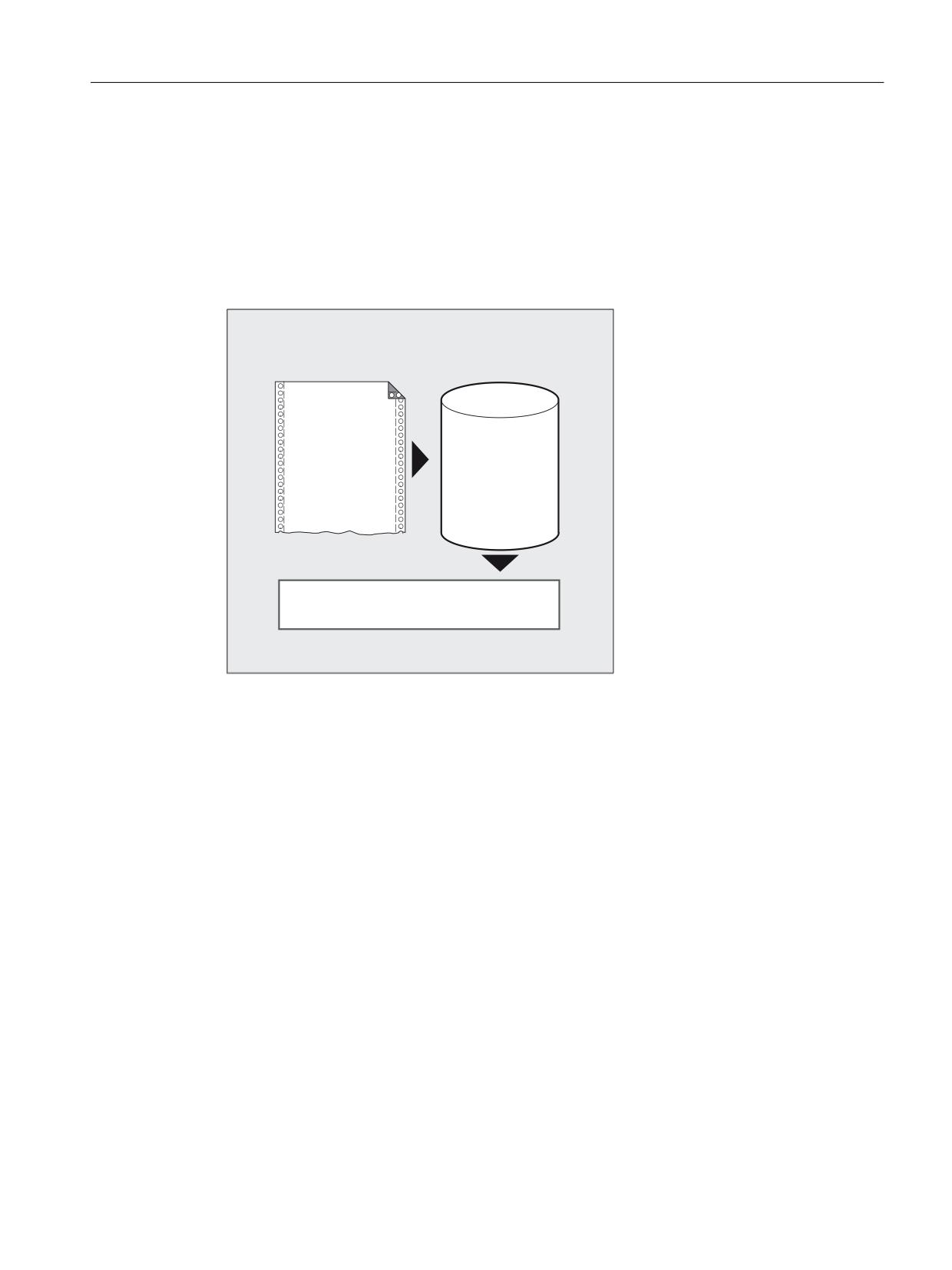
Depending on its expansion level, the control system has a certain quantity of so-called
preprocessing memory in which prepared blocks are stored prior to program execution and
then output as high-speed block sequences while machining is in progress. These sequences
allow short paths to be traversed at a high velocity. Provided that there is sufficient residual
control time available, the preprocessing memory is always filled.
3UHSUR
1& SURJUDP
FHVVLQJ
PHPRU\
3URGXFWLRQ SURFHGXUH IDVW EORFN VHTXHQFH
Designate machining step
The beginning and end of the machining step to be buffered in the preprocessing memory are
identified in the part program with "STOPFIFO" and "STARTFIFO" respectively. The
processing of the preprocessed and buffered blocks starts only after the "STARTFIFO"
command or if the preprocessing memory is full.
Automatic preprocessing memory control
Automatic preprocessing memory control is called with the "FIFOCTRL" command.
"FIFOCTRL" acts initially just like "STOPFIFO". Whatever the programming, processing will
not start until the preprocessing memory is full. However, the response to the emptying of the
preprocessing memory does differ: With "FIFOCTRL", the path velocity is reduced increasingly
once the fill level reaches 2/3 in order to prevent complete emptying and deceleration to
standstill.
Job Planning
Programming Manual, 12/2018, A5E40869460B AB
515
Path traversing behavior
12.6 Program sequence with preprocessing memory (STOPFIFO, STARTFIFO, FIFOCTRL, STOPRE)
Preprocessing stop
Programming the "STOPRE" command in a block will stop block preprocessing and buffering.
The following block is not executed until all preprocessed and saved blocks have been
executed in full. The preceding block is halted in exact stop (as with G9).
NOTICE
Program abort
If tool offset or spline interpolations are active, a "STOPRE" command should not be
programmed, as this will lead to contiguous block sequences being interrupted.
Syntax
Table 12-1
Identify machining step:
STOPFIFO
STARTFIFO
Table 12-2
Automatic preprocessing memory control:
FIFOCTRL
Table 12-3
Preprocessing stop:
STOPRE
Note
The "STOPFIFO", "STARTFIFO", "FIFOCTRL" and "STOPRE" commands must be
programmed in their own block.
Job Planning
516
Programming Manual, 12/2018, A5E40869460B AB

Path traversing behavior
12.6 Program sequence with preprocessing memory (STOPFIFO, STARTFIFO, FIFOCTRL, STOPRE)
Meaning
STOPFIFO:
"STOPFIFO" identifies the start of a machining step to be buffered in the prepro-
cessing memory. "STOPFIFO" stops processing and fills the preprocessing mem-
ory until:
● "STARTFIFO" or "STOPRE" is recognized
or
● The preprocessing memory is full
or
● The end of the program is reached
STARTFIFO:
"STARTFIFO" starts rapid processing of the machining step; the preprocessing
memory is filled in parallel to this.
FIFOCTRL:
Activation of automatic preprocessing memory control
STOPRE:
Stop preprocessing
Note
The preprocessing memory is not filled or filling is interrupted if the machining step contains
commands that require unbuffered operation (search for reference, measuring functions, etc.).
Note
The control generates an internal preprocessing stop in the event of access to status data
($SA...).
Example: Stop preprocessing
Program code
Comment
N30 MEAW=1 G1 F1000 X100 Y100 Z50
; Measurement block with probe at first
measuring input and linear interpola-
tion.
N40 STOPRE
; Preprocessing stop.
Job Planning
Programming Manual, 12/2018, A5E40869460B AB
517
Path traversing behavior
12.7 Defining a stop delay range (DELAYFSTON, DELAYFSTOF)
12.7
Defining a stop delay range (DELAYFSTON, DELAYFSTOF)
The predefined DELAYFSTON and DELAYFSTOF procedures are used to define a
conditionally interruptible range in the part program (stop delay range).
Note
DELAYFSTON and DELAYFSTOF are not permitted in synchronized actions!
Syntax
DELAYFSTON
DELAYFSTOF
Meaning
DELAYFSTON:
Defining the start of a stop delay range
Alone in the block:
Yes
DELAYFSTOF:
Define the end of the stop delay area
Alone in the block:
Yes
Programming example
The following program block is repeated in a loop:
Program code
N99 MY_LOOP:
N100 G0 Z200
N200 G0 X0 Z200
N300 DELAYFSTON
N400 G33 Z5 K2 M3 S1000
N500 G33 Z0 X5 K3
N600 G0 X100
N700 DELAYFSTOF
N800 GOTOB MY_LOOP
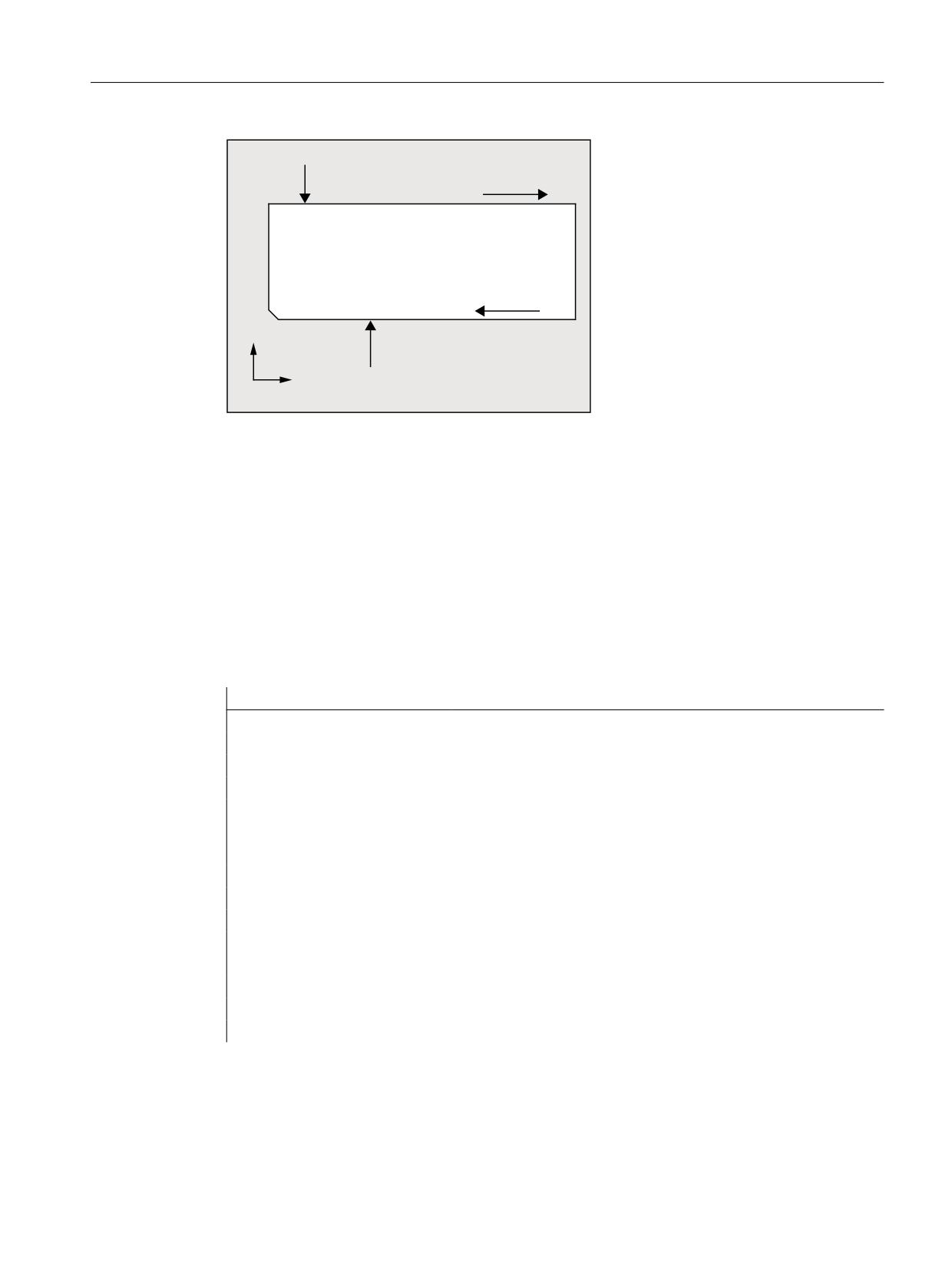
In the following diagram it can be seen that the user pressed "Stop" in the stop delay range,
and the NC started braking outside the stop delay range, i.e. in block N100. That causes the
NC to stop at the beginning of N100.
Job Planning
518
Programming Manual, 12/2018, A5E40869460B AB
Path traversing behavior
12.7 Defining a stop delay range (DELAYFSTON, DELAYFSTOF)
1& VWRSSW
1
* =
1
* ;
1
* ; =
1
*
=
;
1
*
=
;
6WRS EXWWRQ
6WRS EXWWRQ GXULQJ D *
=
PDFKLQLQJ
Additional information
End of subprogram
DELAYFSTOF is activated implicitly at the end of the subprogram in which DELAYFSTON is
called.
Nesting
If subprogram 1 calls subprogram 2 in a stop delay area, the whole of subprogram 2 is a stop
delay area. In particular, DELAYFSTOF in subprogram 2 has no effect.
Example:
Program code
Comment
N10010 DELAYFSTON
; Blocks with N10xxx program level 1.
N10020 R1 = R1 + 1
N10030 G4 F1
; Stop delay area starts.
N10040 subprogram2
; Interpretation of subprogram 2.
N20010 DELAYFSTON
; Ineffective, repeated start, 2nd level.
N20020 DELAYFSTOF
; Ineffective, end at another level.
N20030 RET
N10050 DELAYFSTOF
; Stop delay end of range at the same level.
N10060 R2 = R2 + 2
N10070 G4 F1
; Stop delay area ends. From now, stops act immediately.
Job Planning
Programming Manual, 12/2018, A5E40869460B AB
519
Path traversing behavior
12.7 Defining a stop delay range (DELAYFSTON, DELAYFSTOF)
System variables
The following system variables can be queried to determine whether part program processing
is currently in a stop delay area:
● in the part program with $P_DELAYFST
● in synchronized actions with $AC_DELAYFST
Value
Meaning
0
Delay stop range not active
1
Delay stop area active
Job Planning
520
Programming Manual, 12/2018, A5E40869460B AB
Path traversing behavior
12.8 Prevent program position for SERUPRO (IPTRLOCK, IPTRUNLOCK)
12.8
Prevent program position for SERUPRO (IPTRLOCK, IPTRUNLOCK)
For some complicated mechanical situations on the machine it is necessary to the stop block
search SERUPRO.
By using a programmable interruption pointer it is possible to intervene before an untraceable
point with "Search at point of interruption".
It is also possible to define untraceable sections in part program sections that the NC cannot
yet re-enter. When the program is interrupted, the NC notes the last block that was processed
that can then be searched for via the HMI user interface.
Syntax
IPTRLOCK
IPTRUNLOCK
The commands are located in a part program line and allow a programmable interruption
pointer
Meaning
IPTRLOCK:
Start of untraceable program section
IPTRUNLOCK:
End of untraceable program section
Both commands are only permitted in part programs, but not in synchronous actions.
Example
Nesting of untraceable program sections in two program levels with implicit "IPTRUNLOCK".
Implicit "IPTRUNLOCK" in subprogram 1 ends the untraceable section.
Program code
Comment
N10010 IPTRLOCK()
N10020 R1 = R1 + 1
N10030 G4 F1
; Hold block of the search-suppressed program sec-
tion starts.
N10040 subprogram2
; Interpretation of subprogram 2.
N20010 IPTRLOCK ()
; Ineffective, repeated start.
N20020 IPTRUNLOCK ()
; Ineffective, end at another level.
N20030 RET
N10060 R2 = R2 + 2
N10070 RET
; End of search-suppressed program section.
N100 G4 F2
; Main program is continued.
The interruption pointer then produces an interruption at 100 again.
Job Planning
Programming Manual, 12/2018, A5E40869460B AB
521
Path traversing behavior
12.8 Prevent program position for SERUPRO (IPTRLOCK, IPTRUNLOCK)
Further information
Acquiring and finding untraceable sections
Untraceable program sections are identified with language commands "IPTRLOCK" and
"IPTRUNLOCK".
Command "IPTRLOCK" freezes the interruption pointer at a single block executable in the
main run (SB1). This block will be referred to as the hold block below. If the program is aborted
after "IPTRLOCK", this hold block can be searched for from the HMI user interface.
Continuing from the current block
The interruption pointer is placed on the current block with "IPTRUNLOCK" as the interruption
point for the following program section.
Once the search target is found a new search target can be repeated with the hold block.
An interrupt pointer edited by the user must be removed again via the HMI.
Rules for nesting
The following points govern the interaction between language commands "IPTRLOCK" and
"IPTRUNLOCK" with nesting and the subprogram end.
1. "IPTRLOCK" is activated implicitly at the end of the subprogram in which "IPTRUNLOCK"
is called.
2. "IPTRLOCK" in an untraceable section has no effect.
3. If subprogram 1 calls subprogram 2 in an untraceable section, the whole of subprogram 2
remains untraceable. "IPTRUNLOCK" in particular has no effect in subprogram 2.
For more information, see
/FB1/ Function Manual, Basic Functions; Mode Group, Channel, Program Operation Mode
(K1).
System variable
An untraceable section can be detected in the part program with "$P_IPTRLOCK".
Automatic interrupt pointer
The automatic interrupt pointer automatically defines a previously defined coupling type as
untraceable. Using machine data, for the
● Electronic gear for "EGON"
● Axial master value coupling for "LEADON"
the automatic interrupt pointer is activated. If the programmed interrupt pointer and the
automatic interrupt pointer that can be activated via machine data overlap, then the largest
possible untraceable section will be generated.
Job Planning
522
Programming Manual, 12/2018, A5E40869460B AB
Path traversing behavior
12.9 Repositioning to the contour (REPOSA, REPOSL, REPOSQ, REPOSQA, REPOSH, REPOSHA, DISR,
DISPR, RMIBL, RMBBL, RMEBL, RMNBL)
12.9
Repositioning to the contour (REPOSA, REPOSL, REPOSQ,
REPOSQA, REPOSH, REPOSHA, DISR, DISPR, RMIBL, RMBBL,
RMEBL, RMNBL)
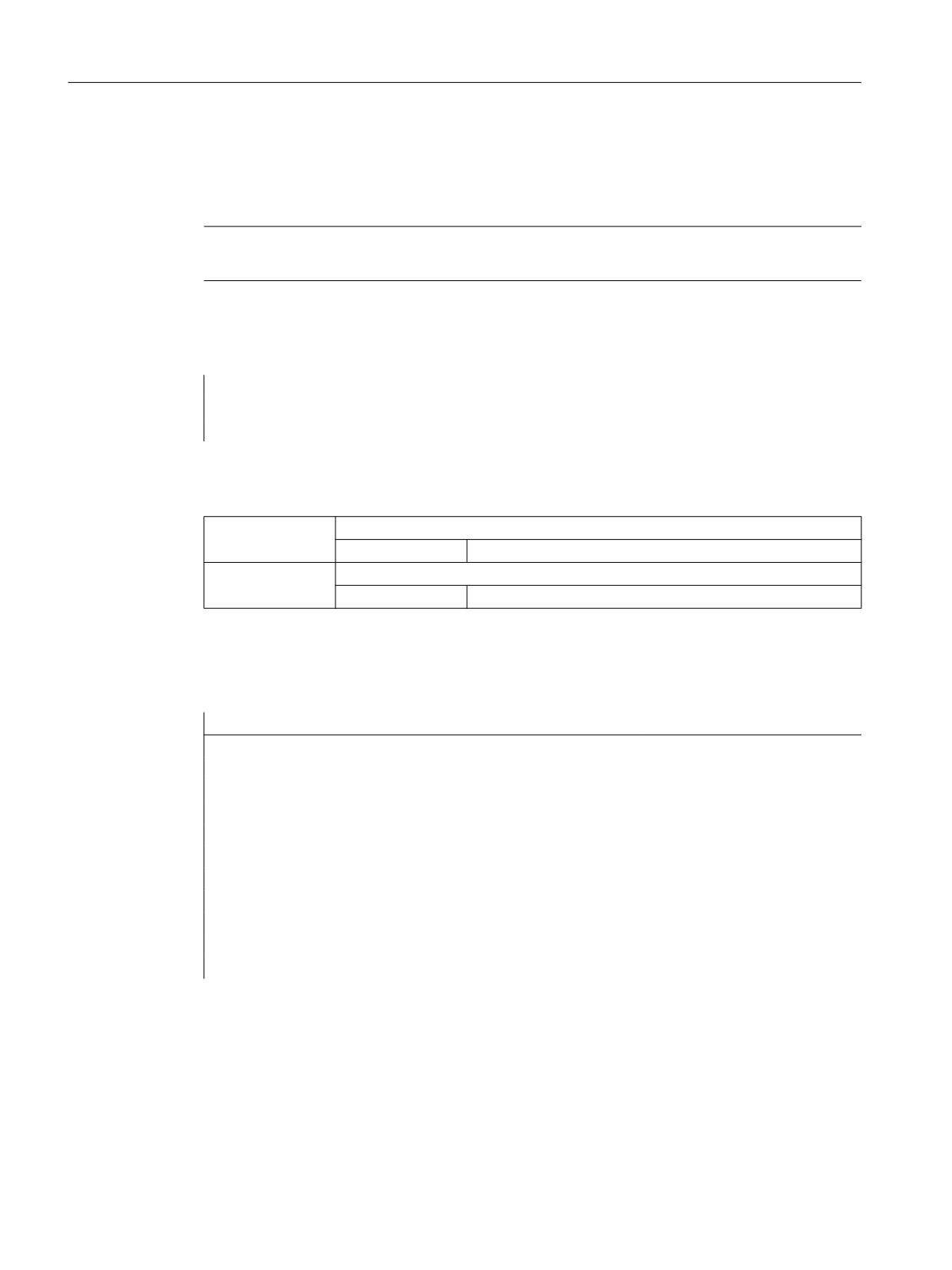
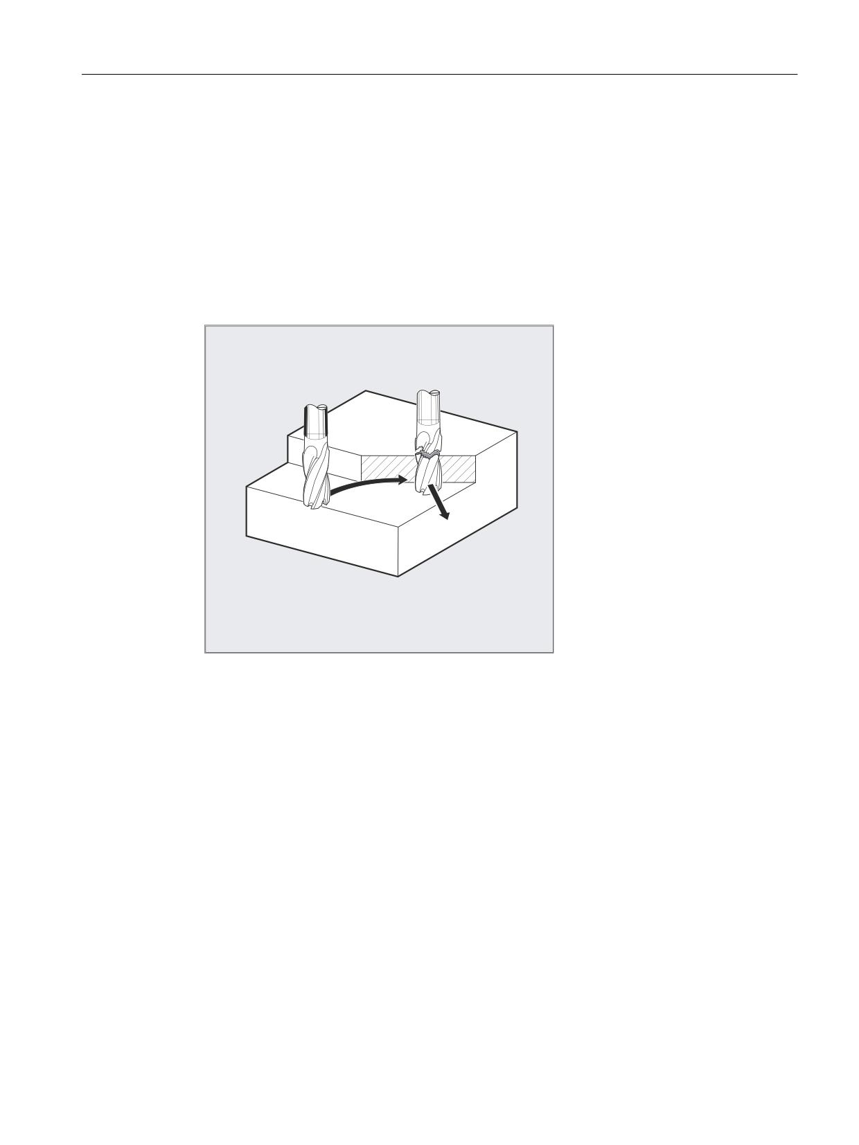
If you interrupt the program run and retract the tool during the machining operation - because,
for example, the tool has broken or you wish to measure the workpiece - you can reposition
at any selected point on the contour under control by the program.
The command REPOS acts in an ASUB as a subprogram return (e.g. M17). The following blocks
are not executed. For information on interrupting program runs, see also "Interrupt routine
(ASUB) (Page 125)."
5(326
Syntax
REPOSA RMIBL DISPR=…
REPOSA RMBBL
REPOSA RMEBL
REPOSA RMNBL
REPOSL RMIBL DISPR=…
REPOSL RMBBL
REPOSL RMEBL
REPOSL RMNBL
REPOSQ RMIBL DISPR=… DISR=…
REPOSQ RMBBL DISR=…
REPOSQ RMEBL DISR=…
REPOSQA DISR=…
REPOSH RMIBL DISPR=… DISR=…
REPOSH RMBBL DISR=…
REPOSH RMEBL DISR=…
REPOSHA DISR=…
Job Planning
Programming Manual, 12/2018, A5E40869460B AB
523

Path traversing behavior
12.9 Repositioning to the contour (REPOSA, REPOSL, REPOSQ, REPOSQA, REPOSH, REPOSHA, DISR,
DISPR, RMIBL, RMBBL, RMEBL, RMNBL)
Meaning
Selecting the approach path
REPOSA:
Repositioning to the contour with the geometry axes along a straight line.
All other channel axes are also repositioned.
REPOSL:
Repositioning to the contour with the geometry axes along a straight line.
Other axes have to be programmed explicitly.
REPOSQ DISR=… :
Repositioning to the contour with the geometry axes along a quadrant of
radius DISR.
Other axes have to be programmed explicitly.
REPOSQA DISR=… :
Repositioning to the contour with the geometry axes along a quadrant of
radius DISR.
All other channel axes are also repositioned.
REPOSH DISR=… :
Repositioning to the contour with the geometry axes along a semicircle
of diameter DISR.
Other axes have to be programmed explicitly.
REPOSHA DISR=… :
Repositioning to the contour with the geometry axes along a semi-circle
of radius DISR.
All other channel axes are also repositioned.
Selecting the repositioning point
RMIBL:
Approach interruption point
RMIBL DISPR=…:
Entry point at distance DISPR in mm/inch in front of interruption point
RMBBL:
Approach block start point
RMEBL:
Approach end of block
RMEBL DISPR=… :
Approach block end point at distance DISPR in front of end point
RMNBL:
Approach at nearest path point
A0 B0 C0 :
Axes in which approach is to be made
Note
Compatibility
To remain compatible with older software versions, you can still program the REPOS approach
mode via the modal commands RMI, RMB, RME and RMN. When used within an ASUB, this
should be allocated the attribute SAVE in the PROC statement. Otherwise the modal REPOS
approach mode used in the ASUB will take effect in subsequent REPOS processes, too, if it
deviates from the preset RMI.
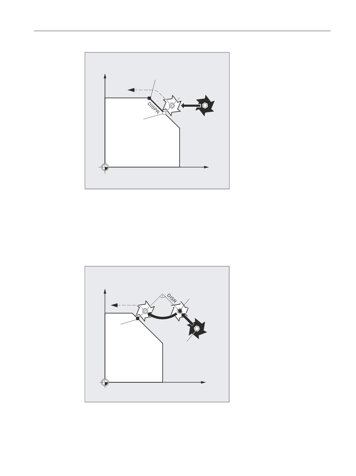
Repositioning to the contour along a straight line, REPOSA, REPOSL
The tool approaches the repositioning point along a straight line.
Example
REPOSL RMIBL DISPR=6 F400
Job Planning
524
Programming Manual, 12/2018, A5E40869460B AB
Path traversing behavior
12.9 Repositioning to the contour (REPOSA, REPOSL, REPOSQ, REPOSQA, REPOSH, REPOSHA, DISR,
DISPR, RMIBL, RMBBL, RMEBL, RMNBL)
<
,QWHUUXSWLRQ SRLQW
5(326/
%ORFN VWDUW SRLQW
;
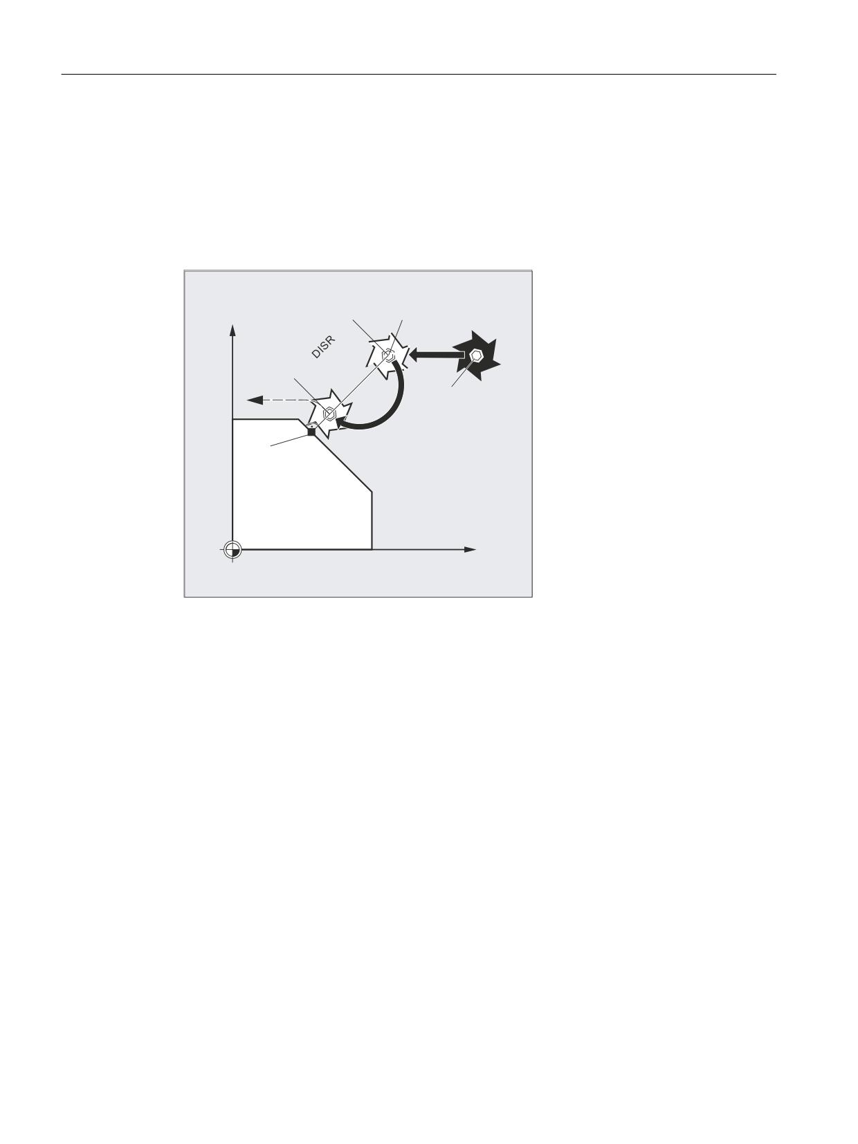
Repositioning to the contour along a quadrant, REPOSQ, REPOSQA
The tool approaches the repositioning point along a quadrant with a radius of DISR=…. The
control automatically calculates the necessary intermediate point between the start and
repositioning point.
Example
REPOSQ RMIBL DISR=10 F400
<
,QWHUPHGLDWH
SRLQW
4
(32 6
5
%ORFN VWDUW SRLQW
6WDUW SRLQW
;
Job Planning
Programming Manual, 12/2018, A5E40869460B AB
525
Path traversing behavior
12.9 Repositioning to the contour (REPOSA, REPOSL, REPOSQ, REPOSQA, REPOSH, REPOSHA, DISR,
DISPR, RMIBL, RMBBL, RMEBL, RMNBL)
Repositioning to the contour along a semicircle, REPOSH, REPOSHA
The tool approaches the repositioning point along a semi-circle with a diameter of DISR=….
The control automatically calculates the necessary intermediate point between the start and
repositioning point.
Example
REPOSH RMIBL DISR=20 F400
,QWHUPHGLDWH SRLQW
<
6WDUW SRLQW
%ORFN VWDUW SRLQW
;
Specifying the repositioning point (not for SERUPRO approaching with RMNBL)
With reference to the NC block in which the program run has been interrupted, it is possible
to select one of three different repositioning points:
● RMIBL, interruption point
● RMBBL, block start point or last end point
● RMEBL, block end point
Job Planning
526
Programming Manual, 12/2018, A5E40869460B AB
Path traversing behavior
12.9 Repositioning to the contour (REPOSA, REPOSL, REPOSQ, REPOSQA, REPOSH, REPOSHA, DISR,
DISPR, RMIBL, RMBBL, RMEBL, RMNBL)
<
%ORFN HQG SRLQW
,QWHUUXSWLRQ SRLQW
50(%/
%ORFN VWDUW
50,%/
SRLQW
50%%/
;
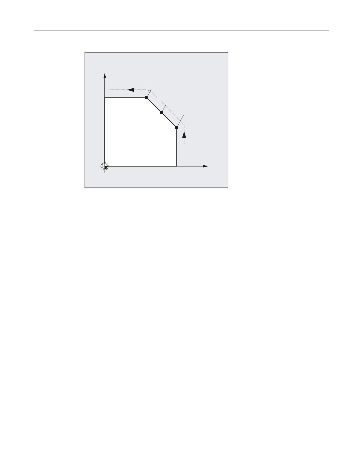
RMIBL DISPR=… or RME DISPR=… allows you to select a repositioning point which lies
before the interruption point or the block end point.
DISPR=… allows you to describe the contour distance in mm/inch between the repositioning
point and the interruption before the end point. Even for high values, this point cannot be further
away than the block start point.
If no DISPR=… command is programmed, then DISPR=0 applies and with it the interruption
point (with RMIBL) or the block end point (with RMEBL).
DISPR sign
The sign of DISPR is evaluated. In the case of a plus sign, the behavior is as previously.
In the case of a minus sign, approach is behind the interruption point or, with RMBBL, behind
the block start point.
The distance between interruption point and approach point depends on the value of DISPR.
Even for higher values, this point can lie in the block end point at the maximum.
Application example:
A sensor will recognize the approach to a clamp. An ASUB is initiated to bypass the clamp.
Afterwards, a negative DISPR is repositioned on one point behind the clamp and the program
is continued.
Job Planning
Programming Manual, 12/2018, A5E40869460B AB
527
Path traversing behavior
12.9 Repositioning to the contour (REPOSA, REPOSL, REPOSQ, REPOSQA, REPOSH, REPOSHA, DISR,
DISPR, RMIBL, RMBBL, RMEBL, RMNBL)
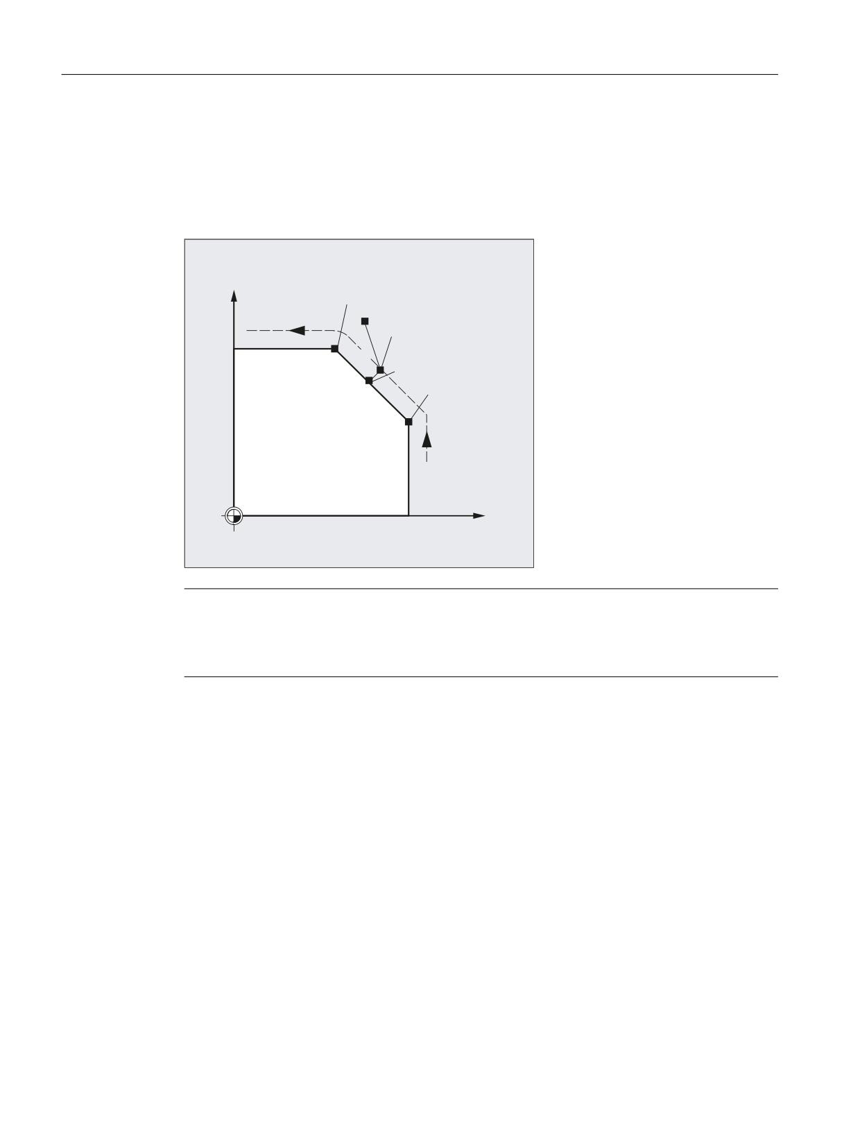
SERUPRO approach with RMNBL
If an abort is forced during machining at any position, the shortest path from the abort point is
approached with SERUPRO approach and RMNBL so that afterward only the distance-to-go
is processed. The user starts a SERUPRO process at the interruption block and uses the JOG
keys to move in front of the problem component of the target block.
%ORFN HQG SRLQW
<
$FWXDO SRVLWLRQ GXULQJ EORFN
VHDUFK
3RVLWLRQ UHDFKHG
ZLWK -2* NH\V
50(%/
6(58352 DSSURDFK
501%/
%ORFN VWDUW
SRLQW
50,%/
50%%/
;
Note
SERUPRO
For SERUPRO, RMIBL and RMBBL are identical. RMNBL is not only limited to SERUPRO,
but is generally valid.
Job Planning
528
Programming Manual, 12/2018, A5E40869460B AB
Path traversing behavior
12.9 Repositioning to the contour (REPOSA, REPOSL, REPOSQ, REPOSQA, REPOSH, REPOSHA, DISR,
DISPR, RMIBL, RMBBL, RMEBL, RMNBL)
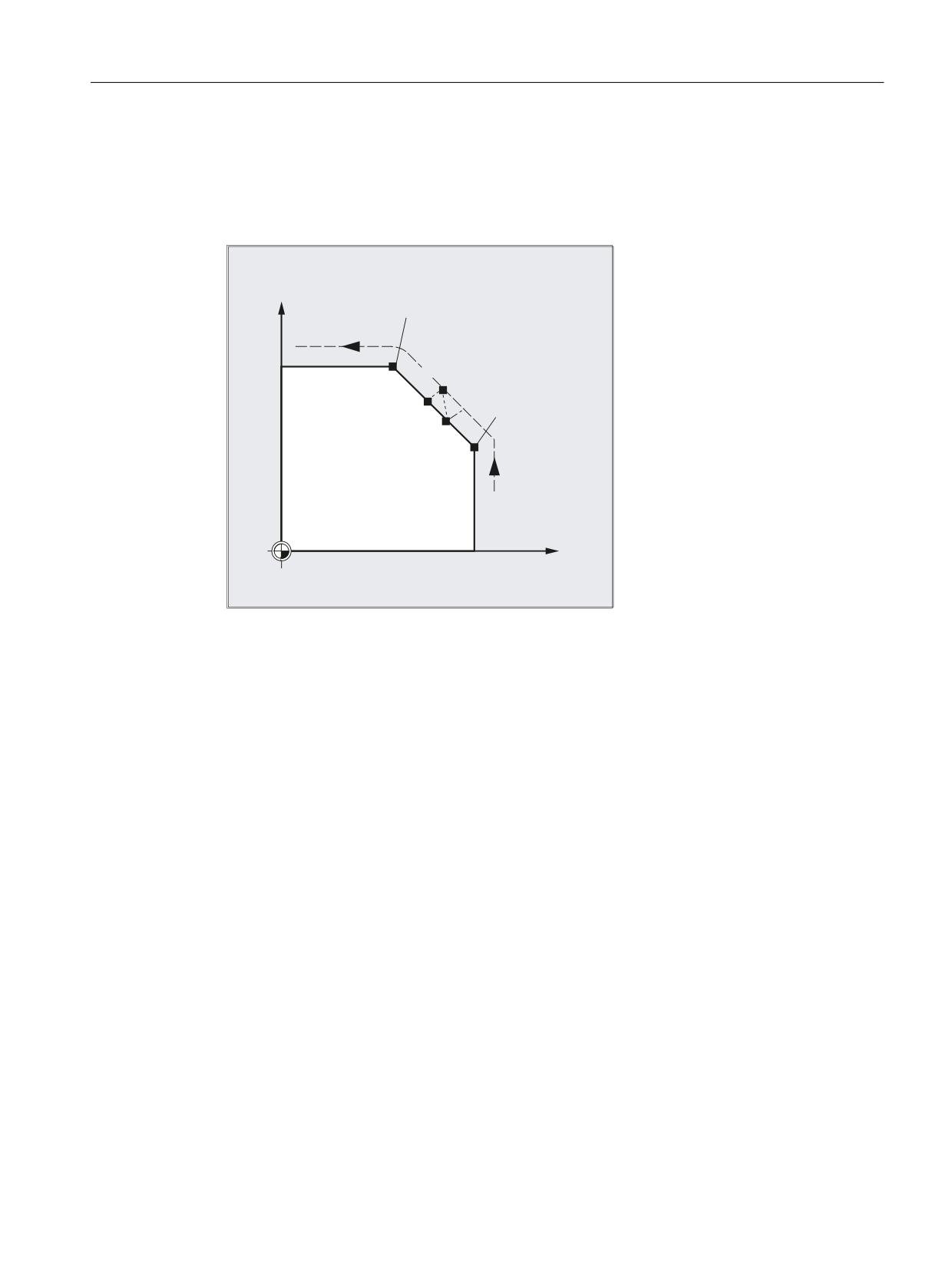
Approach from the nearest path point RMNBL
When REPOSA is interpreted, the repositioning block with RMNBL is not started again in full
after an interruption, but only the distance-to-go processed. The nearest path point of the
interrupted block is approached.
<
%ORFN HQG SRLQW
50(%/
5HSRVLWLRQLQJ
$683
501%/
%ORFN VWDUW
50,%/
SRLQW
50%%/
;
Status for the valid REPOS mode
The valid REPOS mode of the interrupted block can be read with synchronized actions and
variable $AC_ REPOS_PATH_MODE:
0
Approach not defined
1
RMBBL: Approach to beginning
2
RMIBL: Approach to point of interruption
3
RMEBL: Approach to end of block
4
RMNBL: Approach to next path point of the interrupted block
Approaching with a new tool
The following applies if you have stopped the program run due to tool breakage:
When the new D number is programmed, the machining program is continued with modified
tool offset values at the repositioning point.
Where tool offset values have been modified, it may not be possible to reapproach the
interruption point. In such cases, the point closest to the interruption point on the new contour
is approached (possibly modified by DISPR).
Job Planning
Programming Manual, 12/2018, A5E40869460B AB
529
Path traversing behavior
12.9 Repositioning to the contour (REPOSA, REPOSL, REPOSQ, REPOSQA, REPOSH, REPOSHA, DISR,
DISPR, RMIBL, RMBBL, RMEBL, RMNBL)
<
;
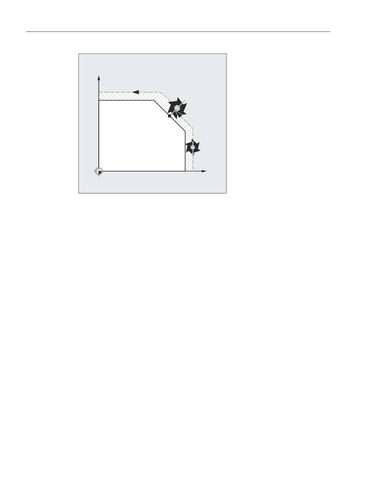
Approach contour
The motion with which the tool is repositioned on the contour can be programmed. Enter zero
for the addresses of the axes to be traversed.
The REPOSA, REPOSQA and REPOSHA commands automatically reposition all axes.
Individual axis names need not be specified.
When the commands REPOSL, REPOSQ and REPOSH are programmed, all geometry axes
are traversed automatically, i.e. they do not have to be specified in the command. All other
axes must be specified in the commands.
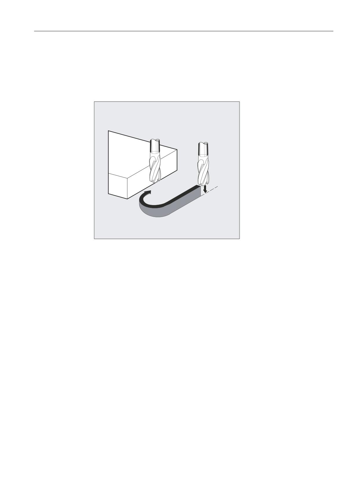
The following applies to the REPOSH and REPOSQ circular motions:
The circle is traversed in the specified working planes G17 to G19.
If you specify the third geometry axis (infeed direction) in the approach block, the repositioning
point is approached along a helix in case the tool position and programmed position in the
infeed direction do not coincide.
Job Planning
530
Programming Manual, 12/2018, A5E40869460B AB
Path traversing behavior
12.9 Repositioning to the contour (REPOSA, REPOSL, REPOSQ, REPOSQA, REPOSH, REPOSHA, DISR,
DISPR, RMIBL, RMBBL, RMEBL, RMNBL)
In the following cases, there is an automatic switchover to linear approach REPOSL:
● You have not specified a value for DISR.
● No defined approach direction is available (program interruption in a block without travel
information).
● With an approach direction that is perpendicular to the current working plane.
Job Planning
Programming Manual, 12/2018, A5E40869460B AB
531
Path traversing behavior
12.10 Influencing the motion control
12.10
Influencing the motion control
12.10.1
Percentage jerk correction (JERKLIM)
Using the NC command "JERKLIM", the maximum jerk of an axis for path motion - set using
machine data - can be reduced or increased in critical program sections.
Requirement
The acceleration mode SOFT must be active.
Effectiveness
The function is effective:
● In the AUTOMATIC operating modes.
● Only on path axes.
Syntax
JERKLIM[<axis>]=<value>
Meaning
JERKLIM:
Command for jerk correction
<axis>:
Machine axis whose jerk limit value is to be adapted.
<value>:
Percentage correction value, referred to the configured maximum axis jerk for path
motion (MD32431 $MA_MAX_AX_JERK).
Range of values:
1 ... 200
Value 100 does not influence the jerk.
Note
The behavior of JERKLIM at the end of the part program and channel reset is configured with
bit 0 in machine data MD32320 $MA_DYN_LIMIT_RESET_MASK:
● Bit 0 = 0:
The programmed value for JERKLIM is reset to 100% with channel reset/M30.
● Bit 0 = 1:
The programmed value for JERKLIM is retained beyond the channel reset/M30.
Example
Program code
Comment
Job Planning
532
Programming Manual, 12/2018, A5E40869460B AB
Path traversing behavior
12.10 Influencing the motion control
Program code
Comment
N60 JERKLIM[X]=75
; The axis slide in the X direction should only be ac-
celerated/decelerated with a maximum of 75% of the jerk
permissible for the axis.
12.10.2
Percentage velocity correction (VELOLIM)
The maximum possible velocity of an axis or the maximum possible gear-stage-dependent
speed of a spindle set via machine data can be reduce with the VELOLIM command in the
part program or synchronized action.
Effectiveness
The function is effective:
● In the AUTOMATIC operating modes.
● On path and positioning axes.
● On spindles in spindle/axis operations
Syntax
VELOLIM[<axis/spindle>]=<value>
Meaning
VELOLIM:
Command for velocity correction
<axis/spindle>:
Axis or spindle whose velocity or speed limit value should be adapted.
VELOLIM for spindles
Using machine data (MD30455 $MA_MISC_FUNCTION_MASK, bit 6),
when programming in the part program, it can be set as to whether "VE-
LOLIM" is effective independent of whether used as spindle or axis
(bit 6 = 1) - or is able to be programmed separately for each operating mode
(bit 6 = 0). If they are to be separately effective, then the selection is made
using the identifier when programming:
● Spindle identifier S<n> for spindle operating modes
● Axis identifier, e.g. "C", for axis operation
Job Planning
Programming Manual, 12/2018, A5E40869460B AB
533

Path traversing behavior
12.10 Influencing the motion control
<value>:
Percentage correction value
The correction value refers to:
● For axes/spindles in axis operation (MD30455 bit 6 == 0):
To the configured maximum axis velocity
(MD32000 $MA_MAX_AX_VELO).
● For spindles in spindle or axis operation (MD30455 bit 6 == 1):
To the maximum speed of the active gear unit stage
(MD35130 $MA_GEAR_STEP_MAX_VELO_LIMIT[<n>])
Range of values:
1 ... 100
The value 100 does not influence the velocity or speed.
Note
Behavior at the end of the part program and for a channel reset
The behavior of "VELOLIM" at the end of the part program and channel reset can be set via
the machine data: MD32320 $MA_DYN_LIMIT_RESET_MASK, bit 0
Detection of an active speed limitation in spindle operation
A speed limitation via "VELOLIM" (less than 100%) can be detected in spindle operation via
the following system variables:
● $AC_SMAXVELO (maximum possible spindle speed)
● $AC_SMAXVELO_INFO (identifier for the speed-limiting cause)
Examples
Example 1: Velocity limitation, machine axis
Program code
Comment
N70 VELOLIM[X]=80
; The axis slide in the X direction should only be trav-
ersed with a maximum of 80% of the velocity permissible
for the axis.
Example 2: Speed limitation, spindle
Program code
Comment
N05 VELOLIM[S1]=90
; Limiting the maximum speed of spindle 1 to 90% of
1000 rpm.
N50 VELOLIM[C]=45
; Limiting the speed to 45% of 1000 rpm, C is the axis
identifier of S1.
Job Planning
534
Programming Manual, 12/2018, A5E40869460B AB
Path traversing behavior
12.10 Influencing the motion control
Machine data settings for spindle 1 (AX5)
● Maximum speed of gear stage 1 = 1000 rpm:
MD35130 $MA_GEAR_STEP_MAX_VELO_LIMIT[ 1, AX5 ] = 1000
● Programming "VELOLIM" acts together for spindle and axis operation independent of the
programmed identifier:
MD30455 $MA_MISC_FUNCTION_MASK[ AX5 ], bit 6 = 1
12.10.3
Program example for JERKLIM and VELOLIM
The following program presents an application example for the percentage jerk and velocity
limit:
Program code
Comments
N1000 G0 X0 Y0 F10000 SOFT G64
N1100 G1 X20 RNDM=5 ACC[X]=20
ACC[Y]=30
N1200 G1 Y20 VELOLIM[X]=5
; The axis slide in the X direction should
only be traversed with max. 5% of the veloc-
ity permissible for the axis.
JERKLIM[Y]=200
; The axis slide in the Y direction can be
accelerated/decelerated with max. 200% of
the jerk permissible for the axis.
N1300 G1 X0 JERKLIM[X]=2
; The axis slide in the X direction should
only be accelerated/decelerated with max. 2%
of the jerk permissible for the axis.
N1400 G1 Y0
M30
Job Planning
Programming Manual, 12/2018, A5E40869460B AB
535
Path traversing behavior
12.11 Programming contour/orientation tolerance (CTOL, OTOL, ATOL)
12.11
Programming contour/orientation tolerance (CTOL, OTOL, ATOL)
Addresses CTOL, OTOL and ATOL can be used to adapt the machining tolerances -
parameterized using machine and setting data - for compressor functions, smoothing and
orientation smoothing in the part program.
The programmed tolerance values are valid until they are reprogrammed or deleted by
assigning a negative value. Further, they are deleted at the end of the program or a reset The
parameterized tolerance values become effective again after deletion.
Syntax
CTOL=<Value>
OTOL=<Value>
ATOL[<Axis>]=<Value>
Meaning
CTOL:
Address to program the contour tolerance
Applications:
● All compressor functions
● All rounding types except G641 and G644
Preprocessing stop:
No
Effective:
Modal
<Value>:
The value for the contour tolerance is specified as a length.
Type:
REAL
Unit:
inch/mm (dependent on the current dimensions
setting)
Value range:
≥ 0:
Tolerance value
< 0:
The programmed tolerance value is de-
leted
⇒ The tolerance value parameterized in
the machine or setting data becomes ef-
fective again.
OTOL:
Address to program the orientation tolerance
Applications:
● All compressor functions
● ORISON orientation smoothing
● All smoothing types except G641, G644 and OSD
Preprocessing stop:
No
Effective:
Modal
<Value>:
The value for the orientation tolerance is specified as an angle.
Type:
REAL
Unit:
degrees
Value range:
≥ 0:
Tolerance value
< 0:
The programmed tolerance value is de-
leted
⇒ The tolerance value parameterized in
the machine or setting data becomes ef-
fective again.
Job Planning
536
Programming Manual, 12/2018, A5E40869460B AB
Path traversing behavior
12.11 Programming contour/orientation tolerance (CTOL, OTOL, ATOL)
ATOL:
Address for programming an axis-specific tolerance
Applications:
● All compressor functions
● ORISON orientation smoothing
● All smoothing types except G641, G644 and OSD
Preprocessing stop:
No
Effective:
Modal
<Axis>:
Name of the channel axis to which the programmed tolerance will
apply
<Value>:
The value for the axis tolerance will be specified as a length or an
angle dependent on the axis type (linear or rotary axis).
Type:
REAL
Unit:
For linear axes:
inch/mm (dependent on
the current dimensions set-
ting)
For rotary axes:
degrees
Value range:
≥ 0:
Tolerance value
< 0:
The programmed tolerance value is de-
leted
⇒ The tolerance value parameterized in
the machine or setting data becomes ef-
fective again.
Note
The channel-specific tolerance values programmed with CTOL and OTOL have higher priority
than the axis-specific tolerance values programmed with ATOL.
Note
Scaling frames
Scaling frames affect programmed tolerances in the same way as axis positions; in other
words, the relative tolerance remains the same.
Example
Program code
Comment
COMPCAD G645 G1 F10000
; Activate COMPCAD compressor function.
X... Y... Z...
; The machine and setting data is applied here.
X... Y... Z...
X... Y... Z...
CTOL=0.02
; A contour tolerance of 0.02 mm is applied start-
ing from here.
X... Y... Z...
X... Y... Z...
X... Y... Z...
ASCALE X0.25 Y0.25 Z0.25
; A contour tolerance of 0.005 mm is applied start-
ing from here.
Job Planning
Programming Manual, 12/2018, A5E40869460B AB
537
Path traversing behavior
12.11 Programming contour/orientation tolerance (CTOL, OTOL, ATOL)
Program code
Comment
X... Y... Z...
X... Y... Z...
X... Y... Z...
CTOL=-1
; The machine and setting data is applied again
starting from here.
X... Y... Z...
X... Y... Z...
X... Y... Z...
System variables
Reading with preprocessing stop
Using the following system variables, the currently active tolerances can be read in the part
program and synchronized action:
● $AC_CTOL
Channel-specific contour tolerance effective when the actual main run block was
preprocessed.
If no contour tolerance is effective, $AC_CTOL will return the root of the sum of the squares
of the tolerances of the geometry axes.
● $AC_OTOL
Channel-specific orientation tolerance effective when the actual main run block was
preprocessed.
If no orientation tolerance is effective, $AC_OTOL will return the root of the sum of the
squares of the tolerances of the orientation axes during active orientation transformation.
Otherwise, it will return the value "-1."
● $AA_ATOL[<axis>]
Axis-specific contour tolerance effective when the actual main run block was preprocessed.
If no contour tolerance is active, $AA_ATOL[<geometry axis>] returns the contour tolerance
divided by the root of the number of geometry axes.
If an orientation tolerance and an orientation transformation are active
$AA_ATOL[<orientation axis>] will return the orientation tolerance divided by the root of
the number of orientation axes.
Note
If now tolerance values have been programmed, the $A variables are not differentiated enough
to distinguish the tolerance of the individual functions.
Circumstances like this can occur if the machine data and the setting data set different
tolerances for compressor functions, smoothing and orientation smoothing. The system
variables then return the greatest value occurring with the functions that are currently active.
For example, if a compressor function is active with an orientation tolerance of 0.1° and
ORISON orientation smoothing with 1°, the $AC_OTOL variable will return the value "1." If
orientation smoothing is deactivated, $AC_OTOL returns a value value "0.1."
Job Planning
538
Programming Manual, 12/2018, A5E40869460B AB
Path traversing behavior
12.11 Programming contour/orientation tolerance (CTOL, OTOL, ATOL)
Reading without preprocessing stop
Using the following system variables, the currently active tolerances can be read in the part
program:
● $P_CTOL
Currently active channel-specific contour tolerance.
● $P_OTOL
Currently active channel-specific orientation tolerance.
● $PA_ATOL
Currently active axis-specific contour tolerance.
Supplementary conditions
The tolerances programmed with CTOL, OTOL and ATOL also affect functions that indirectly
depend on these tolerances:
● Limiting the chord error in the setpoint value calculation
● The basic functions of the free-form surface mode
The following smoothing functions are not affected by the programming of CTOL, OTOL and
ATOL:
● Smoothing the orientation with OSD
OSD does not use a tolerance, it uses a distance from the block transition.
● Smoothing with G644
G644 is not used for smoothing, it is used for optimizing tool changes and other motion not
involving machining.
● Smoothing with G645
G645 virtually always behaves like G642 and, thus, uses the programmed tolerances. The
tolerance value from machine data MD33120 $MA_PATH_TRANS_POS_TOL is only used
in uniformly tangential block transitions with a jump in curvature, e.g. a tangential circle/
straight line transition. The rounding path at these points may also be located outside the
programmed contour, where many applications are less tolerant. Furthermore, it generally
takes a small, fixed tolerance to compensate for the sort of changes in curvature which
need not concern the NC programmer.
Job Planning
Programming Manual, 12/2018, A5E40869460B AB
539
Path traversing behavior
12.12 Block change behavior with active coupling (CPBC)
12.12
Block change behavior with active coupling (CPBC)
The CPBC command specifies the block change criterion that must be satisfied so that a block
change can be executed in the part program with active coupling.
Syntax
CPBC[<following axis>] = <criterion>
Meaning
CPBC:
Block change criterion with active coupling
<following axis>:
Axis identifier of the following axis
<criterion>:
Block change criterion
Type:
STRING
Value
Meaning: Block change is performed
"NOC"
Irrespective of the coupling status
"IPOSTOP"
For setpoint synchronism
"COARSE"
For actual value synchronism "coarse"
"FINE"
For actual value synchronism "fine"
Example
Program code
; Block change takes place with:
;
- Coupling to following axis X2 == active
;
- Setpoint synchronism == active
CPBC[X2]="IPOSTOP"
Job Planning
540
Programming Manual, 12/2018, A5E40869460B AB
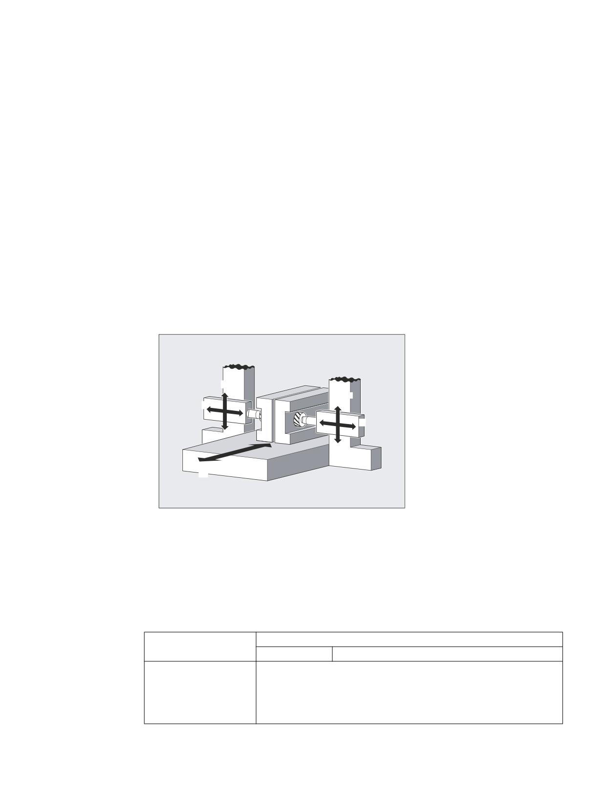
Axis couplings
13
13.1
Coupled motion (TRAILON, TRAILOF)
When a defined leading axis is moved, the coupled motion axes (= following axes) assigned
to it traverse through the distances described by the leading axis, allowing for a coupling factor.
Together, the leading axis and following axis represent coupled axes.
Applications
● Traversal of an axis by means of a simulated axis. The leading axis is a simulated axis and
the coupled axis a real axis. In this way, the real axis can be traversed as a function of the
coupling factor.
● Two-sided machining with two coupled motion groups:
1. leading axis Y, coupled motion axis V
2. leading axis Z, coupled motion axis W
$[LV
<
$[LV
$[LV
9
=
$[LV
:
$[LV
;
Syntax
TRAILON(<following axis>,<leading axis>,<coupling factor>)
TRAILOF(<following axis>,<leading axis>,<leading axis 2>)
TRAILOF(<following axis>)
Meaning
TRAILON:
Command for activating and defining a coupled axis grouping
Effective:
Modal
<following axis>:
Parameter 1: Axis name of trailing axis
Note:
A coupled-motion axis can also act as the leading axis for other coupled-
motion axes. In this way, it is possible to create a range of different coupled
axis groupings.
Job Planning
Programming Manual, 12/2018, A5E40869460B AB
541

Axis couplings
13.1 Coupled motion (TRAILON, TRAILOF)
<leasing axis>:
Parameter 2: Axis name of trailing axis
<coupling factor>:
Parameter 3: Coupling factor
The coupling factor specifies the desired relationship between the paths of
the coupled-motion axis and the leading axis:
<coupling factor> = path of coupled-motion axis/path of leading axis
Type:
REAL
Default:
1
The input of a negative value causes the master and coupled axes to tra-
verse in opposition.
If a coupling factor is not programmed, then coupling factor 1 automatically
applies.
TRAILOF:
Command for deactivating a coupled axis grouping
Effective:
Modal
TRAILOF with 2 parameters deactivates only the coupling to the specified
leading axis:
TRAILOF(<following axis>,<leading axis>)
If a coupled-motion axis has two leading axes, TRAILOF can be called with
three parameters to deactivate both couplings.
TRAILOF(<following axis>,<leading axis>,<leading axis
2>)
Programming TRAILOF without specifying a leading axis produces the
same result:
TRAILOF(<following axis>)
Note
Coupled axis motion is always executed in the base coordinate system (BCS).
The number of coupled axis groupings which may be simultaneously activated is limited only
by the maximum possible number of combinations of axes on the machine.
Job Planning
542
Programming Manual, 12/2018, A5E40869460B AB
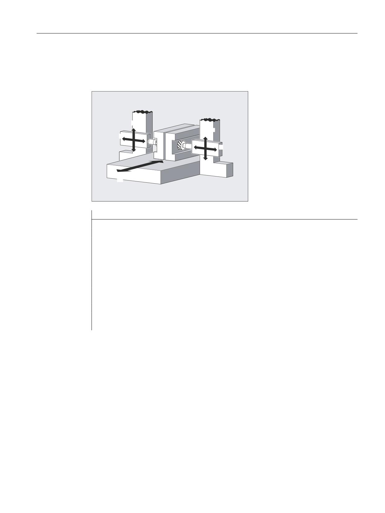
Axis couplings
13.1 Coupled motion (TRAILON, TRAILOF)
Example
The workpiece is to be machined on two sides with the axis configuration shown in the diagram.
To do this, you create two combinations of coupled axes.
$[LV
<
$[LV
$[LV
9
=
$[LV
:
$[LV
;
Program code
Comment
…
N100 TRAILON(V,Y)
; Activation of 1st coupled axis group.
N110 TRAILON(W,Z,-1)
; Activation of 2nd coupled axis grouping, Negative cou-
pling factor: Coupled-motion axis traverses in the oppo-
site direction from leading axis.
N120 G0 Z10
; Infeed of Z and W axes in opposite axial directions.
N130 G0 Y20
; Infeed of Y and V axes in same axis direction.
…
N200 G1 Y22 V25 F200
; Overlaying of a dependent and independent movement of
coupled motion axis V.
…
TRAILOF(V,Y)
; Deactivation of 1st coupled axis grouping.
TRAILOF(W,Z)
; Deactivation of 2nd coupled axis grouping.
Further information
Axis types
A coupled axis grouping can consist of any desired combinations of linear and rotary axes. A
simulated axis can also be defined as a leading axis.
Coupled-motion axes
Up to two leading axes can be assigned simultaneously to a trailing axis. The assignment is
made in different combinations of coupled axes.
A coupled-motion axis can be programmed with the full range of available motion commands
(G0, G1, G2, G3, etc.). The coupled axis not only traverses the independently defined paths,
but also those derived from its leading axes on the basis of coupling factors.
Job Planning
Programming Manual, 12/2018, A5E40869460B AB
543
Axis couplings
13.1 Coupled motion (TRAILON, TRAILOF)
Dynamics limit
The dynamics limit is dependent on the type of activation of the coupled axis grouping:
● Activation in part program
If activation is performed in the part program and all leading axes are active as program
axes in the activated channel, the dynamic response of all coupled-motion axes is taken
into account during traversing of the leading axis to avoid overloading the coupled-motion
axes.
If activation is performed in the part program with leading axes that are not active as
program axes in the activating channel ($AA_TYP ≠ 1), then the dynamic response of the
coupled-motion axes is not taken into account during traversing of the leading axis. This
can cause the overloading of coupled-motion axes with a dynamic response which is less
than that required for the coupling.
● Activation in synchronized action
If activation is performed in a synchronized action, the dynamic response of the coupled-
motion axes is not taken into account during traversing of the leading axis. This can cause
the overloading of coupled-motion axes with a dynamic response which is less than that
required for the coupling.
CAUTION
Axis overload
If a coupled axis grouping is activated:
● In synchronized actions
● In the part program with leading axes that are not program axes in the channel of the
coupled-motion axes
It is the specific responsibility of the user / machine manufacturer to take suitable action
to ensure that the traversing of the leading axis will not cause the overloading of the
coupled-motion axes.
Coupling status
The coupling status of an axis can be checked in the part program with the system variable:
$AA_COUP_ACT[<axis>]
Value
Meaning
0
No coupling active
8
Coupled motion active
Display of distance-to-go of the coupled-motion axis for modulo rotary axes
If the leading and coupled-motion axes are modulo rotary axes, traversing movements in the
leading axis from n * 360° with n = 1, 2, 3 ... , add up in the distance-to-go display of the coupled-
motion axis until the coupling is switched off.
Example: Program section with TRAILON and leading axis B and following axis C
Program code
Comment
TRAILON(C,B,1)
; Activate coupling
G0 B0
; Starting position
; Distance-to-go display at block start:
Job Planning
544
Programming Manual, 12/2018, A5E40869460B AB
Axis couplings
13.1 Coupled motion (TRAILON, TRAILOF)
Program code
Comment
G91 B360
; B=360, C=360
G91 B720
; B=720, C=1080
G91 B360
; B=360, C=1440
Job Planning
Programming Manual, 12/2018, A5E40869460B AB
545
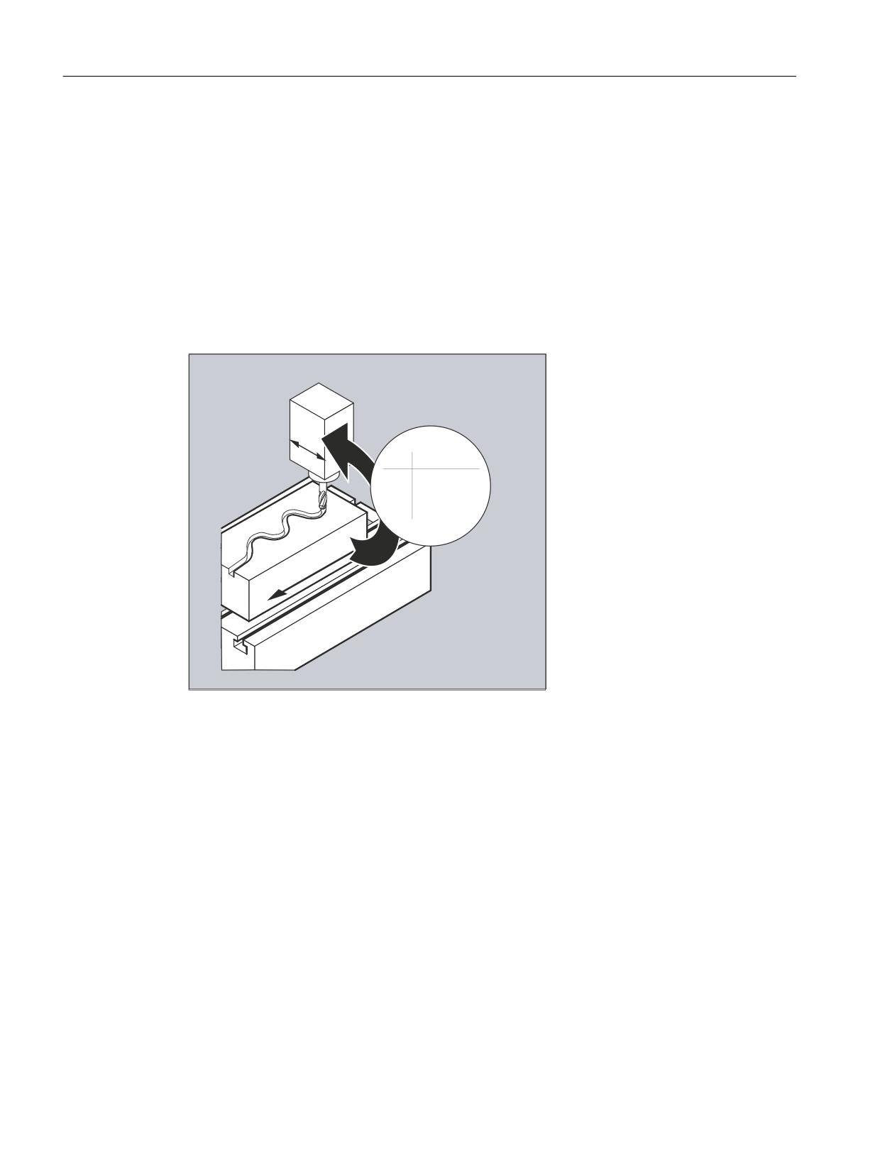
Axis couplings
13.2 Curve tables (CTAB)
13.2
Curve tables (CTAB)
Curve tables can be used to program position and velocity relationships between two axes
(leading and following axis). Curve tables are defined in the part program.
Application
Curve tables replace mechanical cams. The curve table forms the basis for the axial master
value coupling by creating the functional relationship between the leading and the following
value: With appropriate programming, the control calculates a polynomial that corresponds to
the cam from the relative positions of the leading and following axes.
<
[
\
D D D[
D D[
;
13.2.1
Define curve tables (CTABDEF, CATBEND)
A curve table represents a part program or a section of a part program enclosed by CTABDEF
at the start and CTABEND at the end.
Within this part program section, unique following axis positions are assigned to individual
positions of the leading axis using motion operations; these following axis positions are used
as intermediate points when calculating the curve definition in the form of a polynomial up to
the 5th order.
Job Planning
546
Programming Manual, 12/2018, A5E40869460B AB
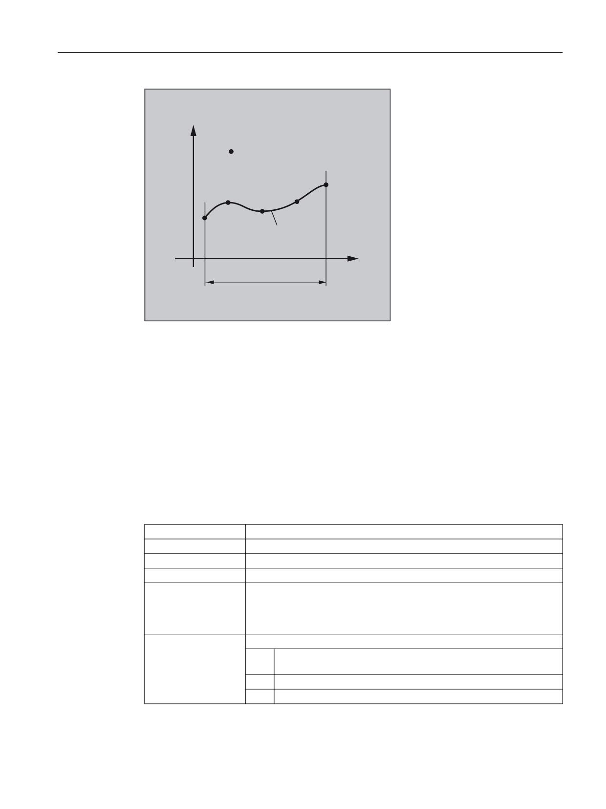
Axis couplings
13.2 Curve tables (CTAB)
6ODYH YDOXH
LQWHUPHGLDWH SRLQW
&XUYH WUDFH
0DVWHU YDOXH
'HILQLWLRQ UDQJH
6WDUWLQJ YDOXH
(QG YDOXH
Requirement
The MD must be configured accordingly to ensure that sufficient memory space is reserved
for the definition of curve tables (→ machine manufacturer).
Syntax
CTABDEF(<following axis>,<leading axis>,<n>,<periodicity>[,<memory
location>])
CTABEND
Meaning
CTABDEF( ):
Start of curve table definition
CTABEND:
End of curve table definition
<following axis>:
Axis whose motion is to be calculated using the curve table
<leasing axis>:
Axis providing the master values for the calculation of the following axis motion
<n>:
Number (ID) of curve table
The number of a curve table is unique and independent of the memory loca-
tion. It is not possible for there to be tables with the same number in the static
and dynamic NC memory.
<periodicity>:
Table periodicity
0
Table is non-periodic (table is processed only once, even for rotary
axes)
1
Table is periodic with regard to the leading axis
2
Table is periodic with regard to leading axis and following axis
Job Planning
Programming Manual, 12/2018, A5E40869460B AB
547

Axis couplings
13.2 Curve tables (CTAB)
<memory
Specification of memory location (optional)
location>:
"SRAM"
The curve table is created in the static NC memory.
"DRAM"
The curve table is created in the dynamic NC memory.
Note:
If a value is not programmed for this parameter, the default memory location
set with MD20905 $MC_CTAB_DEFAULT_MEMORY_TYPE is used.
Note
Overwrite
A curve table is overwritten as soon as its number (<n>) is used in another table definition.
(exception: the curve table is either active in an axis coupling or locked with CTABLOCK). No
warning is output when curve tables are overwritten.
Examples
Example 1: Program section as curve table definition
A program section is to be used unchanged for defining a curve table. The STOPRE command
for preprocessing stop can remain and is reactivated immediately as soon as the program
section is no longer being used for table definition and CTABDEF and CTABEND have been
removed.
Program code
Comment
…
CTABDEF(Y,X,1,1)
; Definition of a curve table.
…
IF NOT ($P_CTABDEF)
STOPRE
ENDIF
…
CTABEND
Job Planning
548
Programming Manual, 12/2018, A5E40869460B AB
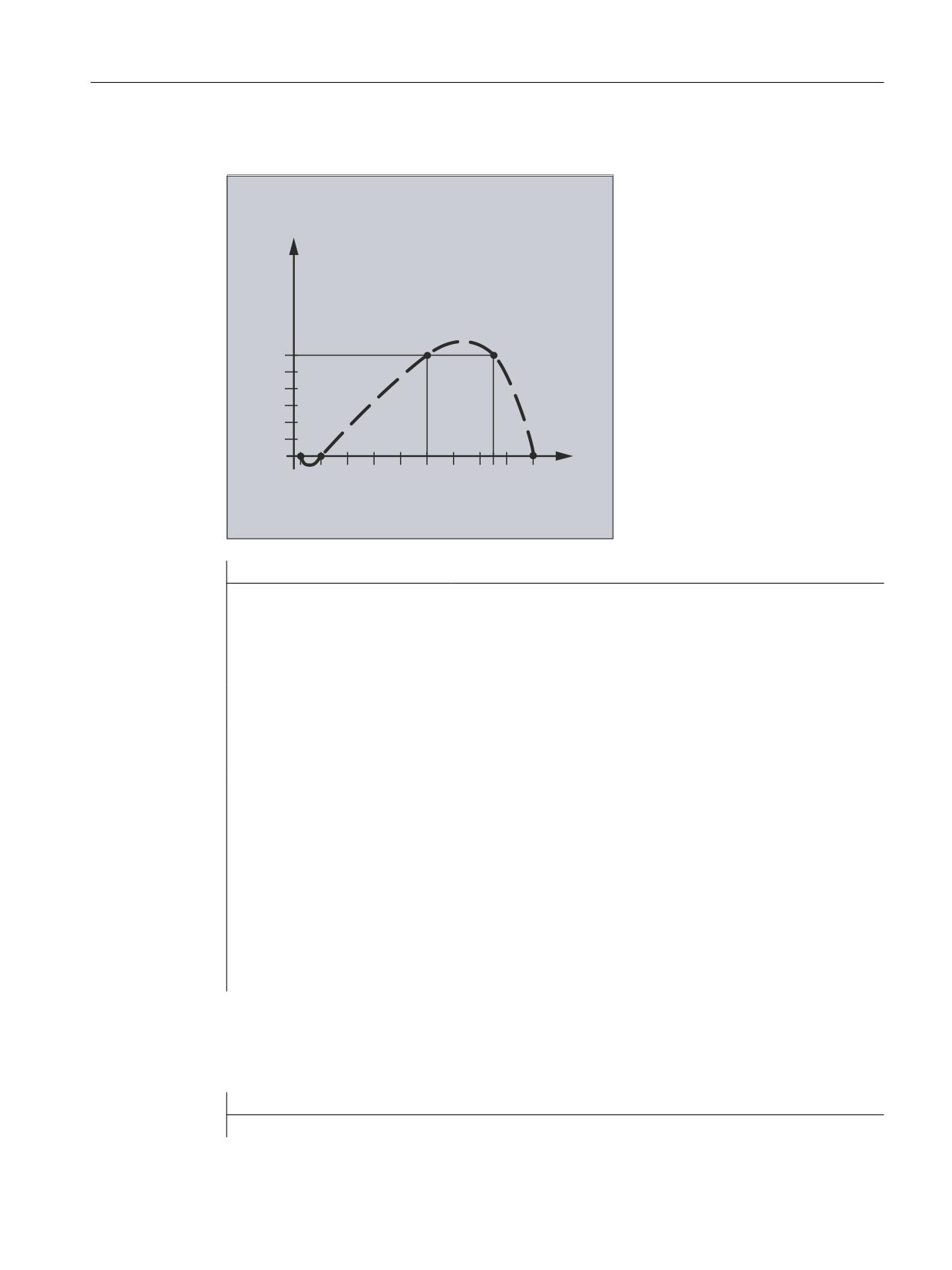
Axis couplings
13.2 Curve tables (CTAB)
Example 2: Definition of a non-periodic curve table
<
;
Program code
Comment
N100 CTABDEF(Y,X,3,0)
; Beginning of the definition of a ;non-periodic curve
table with number 3.
N110 X0 Y0
; 1st motion operation, defines the starting values and
1st intermediate point:
Master value: 0, Following value: 0
N120 X20 Y0
; 2nd interpolation point:
Master value: 0…20, Following value: starting value…0
N130 X100 Y6
; 3rd interpolation point:
Master value: 20…100, Following value: 0…6
N140 X150 Y6
; 4th interpolation point:
Master value: 100…150, Following value: 6…6
N150 X180 Y0
; 5th interpolation point:
Master value: 150…180, Following value: 6…0
N200 CTABEND
; End of the definition. The curve table is generated
in its internal representation as a polynomial of up to
the 5th order. The calculation of the curve definition
with the specified intermediate points is dependent on
the modally selected interpolation type (circular, lin-
ear, spline interpolation). The part program state be-
fore starting the definition is restored.
Example 3: Definition of a periodic curve table
Definition of a periodic curve table with number 2, master value range 0 to 360, following axis
motion from 0 to 45 and back to 0:
Program code
Comment
N10 DEF REAL DEPPOS
Job Planning
Programming Manual, 12/2018, A5E40869460B AB
549
Axis couplings
13.2 Curve tables (CTAB)
Program code
Comment
N20 DEF REAL GRADIENT
N30 CTABDEF(Y,X,2,1)
; Start of definition.
N40 G1 X=0 Y=0
N50 POLY
N60 PO[X]=(45.0)
N70 PO[X]=(90.0) PO[Y]=(45.0,135.0,-90)
N80 PO[X]=(270.0)
N90 PO[X]=(315.0) PO[Y]=(0.0,-135.0,90)
N100 PO[X]=(360.0)
N110 CTABEND
; End of the definition.
;Test of the curve by coupling Y to X:
N120 G1 F1000 X0
N130 LEADON(Y,X,2)
N140 X360
N150 X0
N160 LEADOF(Y,X)
N170 DEPPOS=CTAB(75.0,2,GRADIENT)
; Read the table function for mas-
ter value 75.0.
N180 G0 X75 Y=DEPPOS
; Positioning leading and follow-
ing axes.
;After activating the coupling, no synchronization of the following axis is required.
N190 LEADON(Y,X,2)
N200 G1 X110 F1000
N210 LEADOF(Y,X)
N220 M30
Further Information
Starting and end value of the curve table
The starting value for the beginning of the definition range of the curve table are the first
associated axis positions specified (the first traverse statement) within the curve table
definition. The end value of the definition range of the curve table is determined in accordance
with the last traverse command.
Job Planning
550
Programming Manual, 12/2018, A5E40869460B AB

Axis couplings
13.2 Curve tables (CTAB)
Available language scope
Within the definition of the curve table, you have use of the entire NC language.
Note
The following entries are not permitted in curve table definitions:
● Preprocessing stop
● Jumps in the leading axis movement (e.g. on changing transformations)
● Traverse statement for the following axis only
● Reversal of the leading axis, i.e. position of the leading axis must always be unique
● CTABDEF and CTABEND statement on various program levels.
Effectiveness of modal operations
All modal statements that are made within the curve table definition are invalid when the table
definition is completed. The part program in which the table definition is made is therefore
before and after the table definition in the same state.
Assignments to R-parameters
Assignments to R-parameters in the table definition are reset after CTABEND.
Example:
Program code
Comment
R10=5 R11=20
;R10=5
CTABDEF
G1 X=10 Y=20 F1000
R10=R11+5
;R10=25
X=R10
CTABEND
;R10=5
Activating ASPLINE, BSPLINE, CSPLINE
If an ASPLINE, BSPLINE or CSPLINE is activated within a curve definition table CTABDEF ...
CTABEND, at least a start point should be programmed before this spline activation. Immediate
activation after CTABDEF should be avoided, otherwise the spline will depend on the current
axis position before the curve table definition.
Example:
Program code
CTABDEF(Y,X,1,0)
X0 Y0
ASPLINE
X=5 Y=10
Job Planning
Programming Manual, 12/2018, A5E40869460B AB
551
Axis couplings
13.2 Curve tables (CTAB)
Program code
X10 Y40
CTABEND
Repeated use of curve tables
The functional relationship between the leading axis and the following axis calculated using
the curve table will be retained under the selected table number after the end of the part
program and POWER OFF if the table has been saved to the static NC memory (SRAM).
A table created in the dynamic memory (DRAM) will be deleted on POWER ON and may have
to be regenerated.
Once created, the curve table can be applied to any axis combinations of leading and following
axis and is independent of the axes used to create the curve table.
Overwriting curve tables
A curve table is overwritten as soon as its number is used in another table definition.
Exception: A curve table is either active in an axis coupling or locked with CTABLOCK.
Note
No warning is output when curve tables are overwritten.
Curve table definition active?
The $P_CTABDEF system variable can be used at any time in the part program to check
whether a curve table definition is active.
Revoking the curve table definition
Once the operations relating to the curve table definition have been excluded, the part program
section can be used as a real part program again.
Loading curve tables using "Execution from external source"
If curve tables are executed from an external source, the selection of the size of the reload
buffer (DRAM) in MD18360 $MN_MM_EXT_PROG_BUFFER_SIZE has to support the
simultaneous storage of the entire curve table definition in the reload buffer. If it is not, part
program processing will be canceled with an alarm.
Jumps in the following axis
Depending on the setting in machine data
MD20900 $MC_CTAB_ENABLE_NO_LEADMOTION
, jumps in the following axis may be tolerated if a movement is missing in the leading axis.
13.2.2
Check for presence of curve table (CTABEXISTS)
The CTABEXISTS command can be used to check if a specific curve table number is present
in the NC memory.
Job Planning
552
Programming Manual, 12/2018, A5E40869460B AB
Axis couplings
13.2 Curve tables (CTAB)
Syntax
CTABEXISTS(<n>)
Meaning
CTABEXISTS:
Checks for the presence of curve table number <n> in the static or dynamic NC
memory.
0
Table does not exist
1
Table exists
<n>:
Number (ID) of curve table
13.2.3
Delete curve tables (CTABDEL)
CTABDEL can be used to delete curve tables.
Note
Curve tables that are active in an axis coupling cannot be deleted.
Syntax
CTABDEL(<n>)
CTABDEL(<n>,<m>)
CTABDEL(<n>,<m>,<memory location>)
CTABDEL()
CTABDEL(,,<memory location>)
Meaning
CTABDEL:
Command for deleting curve tables
<n>:
Number (ID) of the curve table to be deleted
When a curve table range CTABDEL(<n>,<m>) is deleted, <n> is used to
specify the number of the first curve table in the range.
<m>:
When a curve table range CTABDEL(<n>,<m>) is deleted, <m> is used to
specify the number of the last curve table in the range.
<m> has to be greater than <n>.
<memory
Specification of memory location (optional)
location>:
In the case of deletion without a memory location being specified, the specified
curve tables are deleted in the static and the dynamic NC memory.
In the case of deletion with a memory location being specified, of the specified
curve tables, only those located in the specified memory location are deleted.
The rest are retained.
"SRAM"
Deletion in the static NC memory
"DRAM"
Deletion in the dynamic NC memory
Job Planning
Programming Manual, 12/2018, A5E40869460B AB
553
Axis couplings
13.2 Curve tables (CTAB)
If CTABDEL is programmed without specification of the curve table to be deleted, then all curve
tables or all curve tables in the specified memory will be deleted:
CTABDEL():
Deletes all curve tables in the static and the dynamic NC memory
CTABDEL(,,"SRAM"):
Deletes all curve tables in the static NC memory
CTABDEL(,,"DRAM"):
Deletes all curve tables in the dynamic NC memory
Note
If, in the case of multiple deletion with CTABDEL(<n>,<m>) or CTABDEL(), at least one of
the of the curve tables to be deleted is active in a coupling, the delete command will not be
executed; in other words, none of the addressed curve tables will be deleted.
13.2.4
Locking curve tables to prevent deletion and overwriting (CTABLOCK,
CTABUNLOCK)
Locks can be set to protect curve tables against unintentional deletion and overwriting. Once
a lock has been set, it can be revoked at any time.
Syntax
Lock:
CTABLOCK(<n>)
CTABLOCK(<n>,<m>)
CTABLOCK(<n>,<m>,<memory location>)
CTABLOCK()
CTABLOCK(,,<memory location>)
Unlock:
CTABUNLOCK(<n>)
CTABUNLOCK(<n>,<m>)
CTABUNLOCK(<n>,<m>,<memory location>)
CTABUNLOCK()
CTABUNLOCK(,,<memory location>)
Meaning
CTABLOCK:
Command for setting a lock to prevent deletion/overwriting
CTABUNLOCK:
Command for revoking a lock to prevent deletion/overwriting
CTABUNLOCK unlocks the curve tables locked with CTABLOCK. Curve tables
which are involved in an active coupling remain locked and cannot be deleted.
The lock with CTABLOCK is unlocked as soon as the lock applied due to the
active coupling is unlocked when the coupling is deactivated. This table can
therefore be deleted. It is not necessary to call CTABUNLOCK again.
Job Planning
554
Programming Manual, 12/2018, A5E40869460B AB
Axis couplings
13.2 Curve tables (CTAB)
<n>:
Number (ID) of the curve table to be locked/unlocked
When a curve table range CTABLOCK(<n>,<m>)/CTABUNLOCK(<n>,<m>)
is locked/unlocked, <n> is used to specify the number of the first curve table
in the range.
<m>:
When a curve table range CTABLOCK(<n>,<m>)/CTABUNLOCK(<n>,<m>)
is locked/unlocked, <m> is used to specify the number of the last curve table
in the range.
<m> has to be greater than <n>.
<memory
Specification of memory location (optional)
location>:
In the case of locking/unlocking without a memory location being specified,
the specified curve tables are locked/unlocked in the static and the dynamic
NC memory.
In the case of locking/unlocking with a memory location being specified, of
the specified curve tables, only those located in the specified memory location
are locked/unlocked. The rest are not locked/unlocked.
"SRAM"
Lock/unlock in the static NC memory
"DRAM"
Lock/unlock in the dynamic NC memory
If CTABLOCK/CTABUNLOCK is programmed without specification of the curve table to be
locked/unlocked, then all curve tables or all curve tables in the specified memory will be locked/
unlocked:
CTABLOCK():
Locks all curve tables in the static and the dynamic NC memory
CTABLOCK(,,"SRAM"):
Locks all curve tables in the static NC memory
CTABLOCK(,,"DRAM"):
Locks all curve tables in the dynamic NC memory
CTABUNLOCK():
Unlocks all curve tables in the static and dynamic NC memory
CTABUNLOCK(,,"SRAM"):
Unlocks all curve tables in the static NC memory
CTABUNLOCK(,,"DRAM"):
Unlocks all curve tables in the dynamic NC memory
13.2.5
Curve tables: Determine table properties (CTABID, CTABISLOCK,
CTABMEMTYP, CTABPERIOD)
These commands can be used to poll important properties of a curve table (table number, lock
state, memory location, periodicity).
Syntax
CTABID(<p>)
CTABID(<p>,<memory location>)
CTABISLOCK(<n>)
CTABMEMTYP(<n>)
TABPERIOD(<n>)
Job Planning
Programming Manual, 12/2018, A5E40869460B AB
555
Axis couplings
13.2 Curve tables (CTAB)
Meaning
CTABID:
Returns the table number entered as the <p>th curve table in the specified
memory.
Example:
CTABID(1,"SRAM") returns the number of the first curve table in the static
NC memory. In this context the first curve table is the curve table with the
highest table number.
Note:
If the sequence of curve tables in the memory changes between consecutive
calls of CTABID, e.g. due to the deletion of curve tables with CTABDEL,
CTABID(<p>,...) can return a different curve table with the same number
<p>.
CTABISLOCK:
Returns the lock state of curve table number <n>:
0
Table is not locked
1
Table is locked by CTABLOCK
2
Table is locked by active coupling
3
Table is locked by CTABLOCK and active coupling
-1
Table does not exist
CTABMEMTYP:
Returns the memory location of curve table number <n>:
0
Table in the static NC memory
1
Table in the dynamic NC memory
-1
Table does not exist
CTABPERIOD:
Returns the periodicity of curve table number <n>:
0
Table is not periodic
1
Table is periodic in the leading axis
2
Table is periodic in the leading and following axes
-1
Table does not exist
<p>:
Entry number in memory
<n>:
Number (ID) of curve table
<memory
Specification of memory location (optional)
location>:
"SRAM"
Static NC memory
"DRAM"
Dynamic NC memory
Note:
If a value is not programmed for this parameter, the default memory location
set with MD20905 $MC_CTAB_DEFAULT_MEMORY_TYPE is used.
13.2.6
Read curve table values (CTABTSV, CTABTEV, CTABTSP, CTABTEP,
CTABSSV, CTABSEV, CTAB, CTABINV, CTABTMIN, CTABTMAX)
The following curve table values can be read in the part program:
● Following axis and leading axis values at the start and end of a curve table
● Following axis values at the start and end of a curve segment
● Following axis value for a leading axis value
Job Planning
556
Programming Manual, 12/2018, A5E40869460B AB

Axis couplings
13.2 Curve tables (CTAB)
● Leading axis value for a following axis value
● Following axis minimum and maximum values
- In the entire definition range of the curve table
or
- In a defined curve table interval
Syntax
CTABTSV(<n>,<gradient>[,<following axis>])
CTABTEV(<n>,<gradient>[,<following axis>])
CTABTSP(<n>,<gradient>[,<leading axis>])
CTABTEP(<n>,<gradient>[,<leading axis>])
CTABSSV(<master value>,<n>,<gradient>[,<following axis>])
CTABSEV(<master value>,<n>,<gradient>[,<following axis>])
CTAB(<master value>,<n>,<gradient>[,<following axis>,<leading axis>]
CTABINV(<following value>,<approximate
value>,<n>,<gradient>[,<following axis>,<leading axis>]
CTABTMIN(<n>[,<following axis>])
CTABTMAX(<n>[,<following axis>])
CTABTMIN(<n>,<a>,<b>[,<following axis>,<leading axis>])
CTABTMAX(<n>,<a>,<b>[,<following axis>,<leading axis>])
Meaning
CTABTSV:
Read following axis value at the start of curve table no. <n>
CTABTEV:
Read following axis value at the end of curve table no. <n>
CTABTSP:
Read leading axis value at the start of curve table no. <n>
CTABTEP:
Read leading axis value at the end of curve table no. <n>
CTABSSV:
Read following axis value at the start of the curve segment belonging to the
specified leading axis value (<master value>)
CTABSEV:
Read following axis value at the end of the curve segment belonging to the
specified leading axis value (<master value>)
CTAB:
Read following axis value for specified leading axis value (<master
value>)
CTABINV:
Read leading axis value for specified following axis value (<following
value>)
CTABTMIN:
Define following axis minimum value:
● In the entire definition range of the curve table
or
● In a defined interval <a> ... <b>
CTABTMAX:
Define following axis maximum value:
● In the entire definition range of the curve table
or
● In a defined interval <a> ... <b>
<n>:
Number (ID) of curve table
<gradient>:
The <gradient> parameter returns the incline of the curve table function
at the calculated position.
Job Planning
Programming Manual, 12/2018, A5E40869460B AB
557