SINUMERIK 840D sl. Service - Functions. Manual (2018-2020)

Detailed description

4.13 Control behavior in specific operating states

Synchronized actions of the ASUB

If the ASUB is not continued with REPOS, the modal and static synchronized actions from the

ASUB remain effective in the part program.

4.13.8

REPOS

In the remainder of the block, the synchronized actions are treated in the same way as in an

interruption block.

Modifications to modal synchronized actions in the asynchronous subprogram are not effective

in the interrupted program.

Polynomial coefficients programmed with FCTDEF are not affected by ASUB and REPOS.

The coefficients from the calling program are applied in the asynchronous subprogram. The

coefficients from the asynchronous subprogram continue to be applied in the calling program.

If positioning motions started from synchronized actions are interrupted by the operating mode

change or start of the interrupt routine, then they are continued with REPOS.

4.13.9

Response to alarms

• If an action of a synchronized action triggers an alarm, this action will be aborted. Other

actions of the synchronized action are processed.

• If a modal synchronized action triggers an alarm, it will be inactive after the interrupt time.

• If a technology cycle generates an alarm with motion stop, it will then be aborted and no

longer processed.

• If an alarm is triggered with motion stop, all axis/spindle motions, which were started by

synchronized actions, will be stopped. Actions without traversing motion are still executed.

• If an alarm is triggered with interpreter stop, it will only have an effect on synchronized

actions after complete execution of the predecoded blocks.

Synchronized actions

130

Function Manual, 10/2020, 6FC5397-5BP40-6BA4

Detailed description

4.14 Diagnostics

4.14

Diagnostics

4.14.1

Displaying the status of synchronized actions

The following information is displayed for diagnosing synchronized actions in the "Synchronized

Actions" window of the "Machine" operating area:

• List of programmed synchronized actions

• Validity and identification number (only for modal synchronized actions)

See Section "Validity, identification number (ID, IDS) (Page 16)"

• Status of synchronized actions

Status

Meaning

Waiting

The condition is being checked in the interpolation cycle.

Active

The action part of the synchronized action is being executed. If the action con-

sists of a technology cycle, the cycle displays the current block number.

Locked

The synchronized action is locked.

See Chapter:

• Coordination via part program and synchronized action (LOCK, UNLOCK,

CANCEL) (Page 123)

• Coordination via PLC (Page 123)

Note

Non-modal synchronized actions can only be identified by their status display. They are only

displayed during execution.

Synchronized actions

Function Manual, 10/2020, 6FC5397-5BP40-6BA4

131

Examples

5.1

Examples of conditions in synchronized actions

Condition

Programming

Path distance-to-go ≤ 10 mm (WCS)

... WHEN $AC_DTEW <= 10 DO ...

Distance-to-go of the X axis ≤ 10 mm (WCS)

... WHEN $AA_DTEW[X]<= 10 DO ...

Path distance to start of block ≥ 20 mm (BCS)

...WHEN $AC_PLTBB >= 20 DO ...

Actual value of the Y axis (MCS) > 10 * SIN(R10)

... WHEN $AA_IM[y] > 10*SIN (R10) DO...

Input 1 changes from 0 to 1

... EVERY $A_IN[1]==1 DO ...

Input 1 == 1

... WHENEVER $A_IN[1]==0 DO ...

5.2

Reading and writing of SD/MD from synchronized actions

Infeed and oscillation for grinding operations

Setting data, whose values remain unchanged during machining, are addressed by name as in

the part program.

Example: Oscillation from synchronized actions

Program code

N610 ID=1 WHENEVER $AA_IM[Z] > $SA_OSCILL_REVERSE_POS1[Z] DO $AC_MARKER[1]=0

; ALWAYS WHEN current position of the oscillating axis in the MCS < start of reversal area 2,

; THEN override of the infeed axis = 0%

N620 ID=2 WHENEVER $AA_IM[Z] < $SA_OSCILL_REVERSE_POS2[Z] - 6 DO

$AA_OVR[X]=0 $AC_MARKER[0]=0

; ALWAYS WHEN current position of the oscillating axis in the MCS == reversal position 1,

; THEN override of the oscillation axis = 0%, override of the infeed axis = 100%

; This cancels the previous synchronized action!

N630 ID=3 WHENEVER $AA_IM[Z] == $SA_OSCILL_REVERSE_POS1[Z] DO

$AA_OVR[Z]=0 $AA_OVR[X]=100

; ALWAYS WHEN distance-to-go of the partial infeed == 0,

; THEN override of the oscillation axis = 100%

; This cancels the previous synchronized action!

N640 ID=4 WHENEVER $AA_DTEPW[X]==0 DO $AA_OVR[Z]=100 $AC_MARKER[0]=1 $AC_MARKER[1]=1

N650 ID=5 WHENEVER $AC_MARKER[0]==1 DO $AA_OVR[X]=0

N660 ID=6 WHENEVER $AC_MARKER[1]==1 DO $AA_OVR[X]=0

Synchronized actions

Function Manual, 10/2020, 6FC5397-5BP40-6BA4

133

Examples

5.2 Reading and writing of SD/MD from synchronized actions

Program code

; WHEN current position of the oscillating axis in the WCS == reversal position 1,

; THEN override of the oscillation axis = 100%, override of the infeed axis = 0%

; This cancels the second synchronized action once!

N670 ID=7 WHEN $AA_IM[Z] == $SA_OSCILL_REVERSE_POS1[Z] DO $AA_OVR[Z]=100 $AA_OVR[X]=0

; Setting data whose value changes during machining (e.g. by means of

; operator input or synchronized action) must be programmed with $$S...:

; Example: Oscillation from synchronized actions with change of the oscillation

; position via the user interface

N610 ID=1 WHENEVER $AA_IM[Z] > $$SA_OSCILL_REVERSE_POS1[Z] DO $AC_MARKER[1]=0

; ALWAYS WHEN current position of the oscillating axis in the MCS < start of reversal area 2,

; THEN override of the infeed axis = 0%

N620 ID=2 WHENEVER $AA_IM[Z] < $$SA_OSCILL_REVERSE_POS2[Z]-6 DO

$AA_OVR[X]=0 $AC_MARKER[0]=0

; ALWAYS WHEN current position of the oscillating axis in the MCS == reversal position 1,

; THEN override of the oscillation axis = 0%, override of the infeed axis = 100%

; This cancels the previous synchronized action!

N630 ID=3 WHENEVER $AA_IM[Z]==$$SA_OSCILL_REVERSE_POS1[Z] DO

$AA_OVR[Z]=0 $AA_OVR[X]=100

; ALWAYS WHEN distance-to-go of the partial infeed == 0,

; THEN override of the oscillation axis = 100%

; This cancels the previous synchronized action!

N640 ID=4 WHENEVER $AA_DTEPW[X]==0 DO $AA_OVR[Z]=100 $AC_MARKER[0]=1 $AC_MARKER[1]=1

N650 ID=5 WHENEVER $AC_MARKER[0]==1 DO $AA_OVR[X]=0

N660 ID=6 WHENEVER $AC_MARKER[1]==1 DO $AA_OVR[X]=0

; WHEN current position of the oscillating axis in the WCS == reversal position 1,

; THEN override of the oscillation axis = 100%, override of the infeed axis = 0%

; This cancels the second synchronized action once!

N670 ID=7 WHEN $AA_IM[Z]==$$SA_OSCILL_REVERSE_POS1[Z]

DO $AA_OVR[Z]=100 $AA_OVR[X]=0

Synchronized actions

134

Function Manual, 10/2020, 6FC5397-5BP40-6BA4

Examples

5.3 Examples of adaptive control

5.3

Examples of adaptive control

General procedure

The following examples use the polynomial evaluation function SYNFCT().

1. Representation of relationship between input value and output value (main run variables in

each case)

2. Definition of this relationship as polynomial with limitations

3. With position offset: Setting the MD and SD

- MD36750 $MA_AA_OFF_MODE (Effect of value assignment for axial override in case of

synchronized actions)

- SD43350 $SA_AA_OFF_LIMIT (optional) (Upper limit of the offset value $AA_OFF in case

of clearance control)

4. Activation of the control in a synchronized action

5.3.1

Clearance control with variable upper limit

Example of polynomial with dynamic upper limit

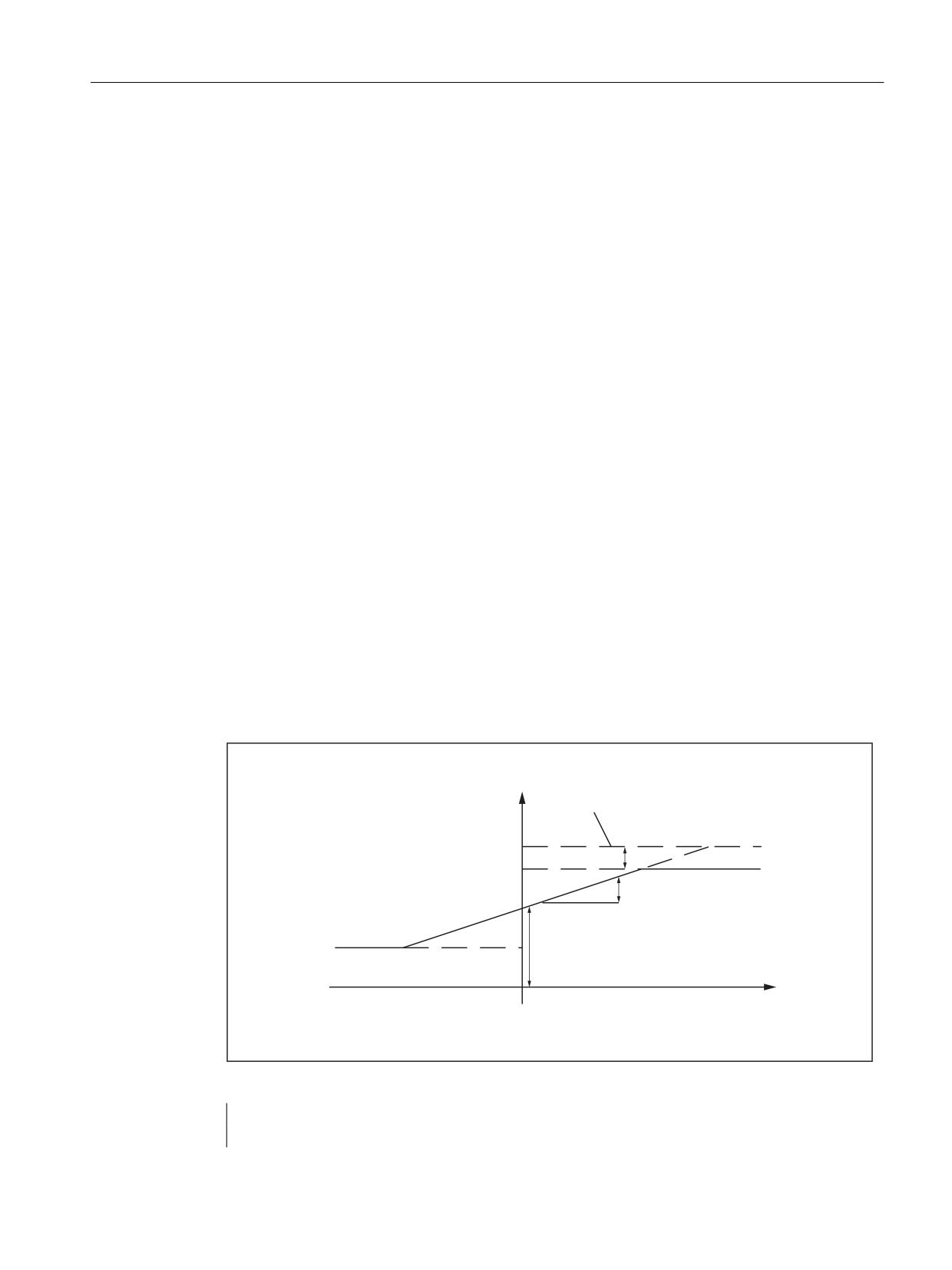
For the purpose of clearance control, the upper limit of the output ($AA_OFF, override value in

axis V) is varied as a function of the spindle override (analog input 1). The upper limit for

polynomial 1 is varied dynamically as a function of analog input 2.

Polynomial 1 is defined directly via system variables:

$$B2))>9@

$GDSWDWLRQ UDQJH RI

XSSHU OLPLW

$&B)&78/> @

$&B)&7 > @

$B,1$> @

Figure 5-1

Clearance control with variable upper limit

$AC_FCTLL[1]=0.2

; Lower limit

$AC_FCTUL[1]=0.5

; Request Value of upper limit

Synchronized actions

Function Manual, 10/2020, 6FC5397-5BP40-6BA4

135

Examples

5.3 Examples of adaptive control

$AC_FCT0[1]=0.35

; Zero passage a

$AC_FCT1[1]=1.5 EX-5

; Pitch a₁

STOPRE

; see following note

STOPRE

; see following note

ID=1 DO $AC_FCTUL[1]=$A_INA[2]*0.1+0.35

;

Adjust upper limit dynamically via

analog input 2,

;

no condition

;

ID=2 DO SYNFCT(1, $AA_OFF[V], $A_INA[1])

;

Clearance control by override of no

condition

;

Note

When system variables are used in the part program, STOPRE must be programmed to ensure

block-synchronous writing. The following is an equivalent notation for polynomial definition:

FCTDEF(1,0.2, 0.5, 0.35, 1.5EX-5).

Synchronized actions

136

Function Manual, 10/2020, 6FC5397-5BP40-6BA4

Examples

5.3 Examples of adaptive control

5.3.2

Feedrate control

Example of adaptive control with an analog input voltage

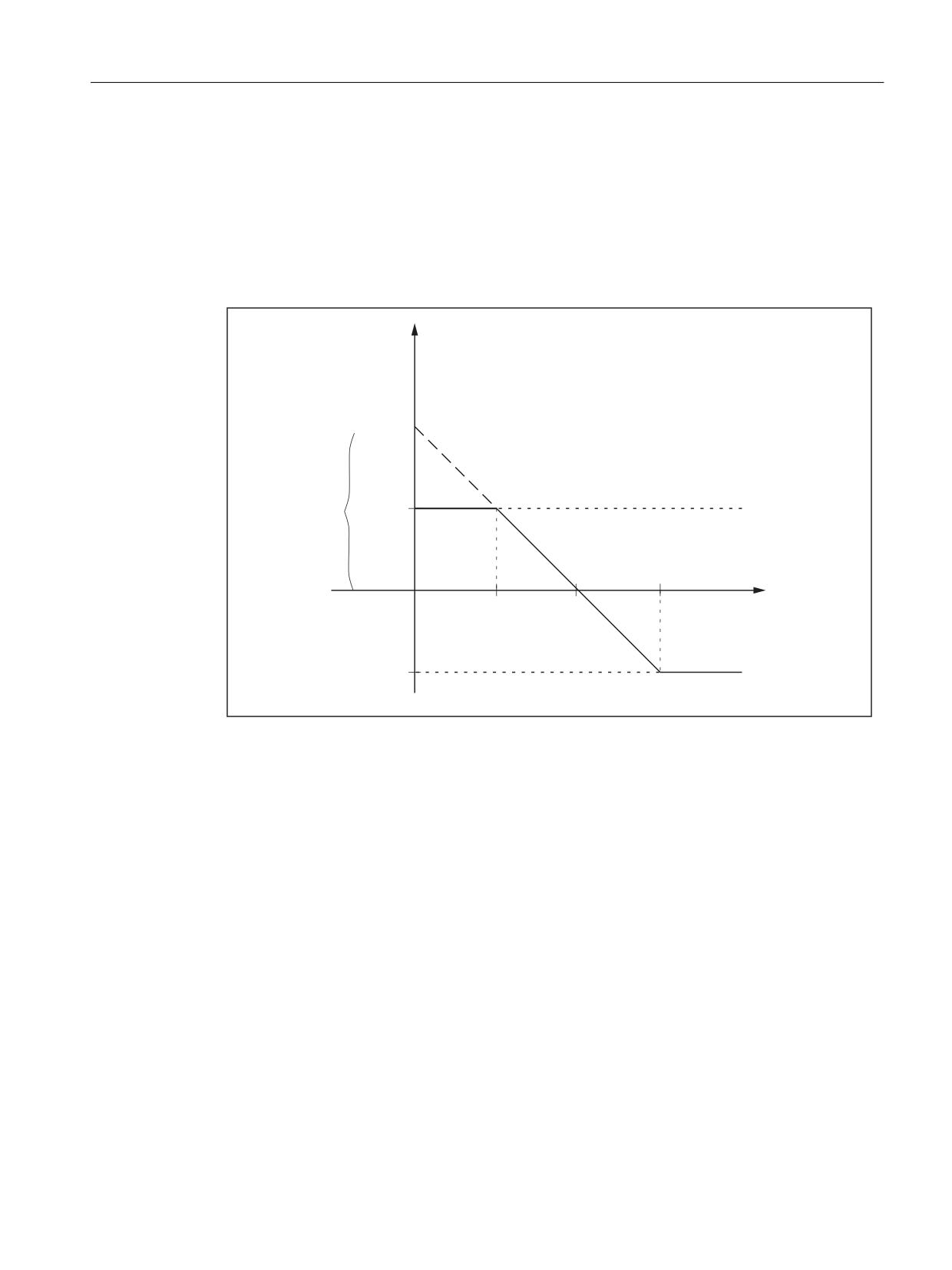
A process quantity (measured via $A_INA[1]) is to be controlled at 2 V using an additive control

factor implemented by a path (or axial) feedrate override. Feedrate override is to be performed

within the range of +100 [mm/min].

3DWK DQG D[LDO

IHHGUDWH RIIVHW

$&B9&

$$B9&>$;@

8QLW

H J PP PLQ

8/,0,7

$QDORJ LQSXW

$B,1$> @

8QLW

//,0,7

Figure 5-2

Diagram illustrating adaptive control

Determining the coefficients:

y = f(x) = a₀ + a₁x +a₂x² + a₃x³

a1 = - 100mm / (1min * 1V)

a1 = - 100% control constant, gradient

a0 = - (-100) * 2 = 200

a2 = 0 (not a square component)

a3 = 0 (not a cubic component)

upper limit = 100

Lower limit = -100

FCTDEF(

Polynomial

LLIMIT,

ULIMIT,

a₀,

; y for x = 0

a₁,

; gradient

Synchronized actions

Function Manual, 10/2020, 6FC5397-5BP40-6BA4

137

Examples

5.3 Examples of adaptive control

; square component

a₃ )

; cubic component

With the values determined above, the polynomial is defined as follows:

FCTDEF(1, -100, 100, 200, -100, 0, 0)

The following synchronized actions can be used to activate the adaptive control function:

for the axis feedrate:

ID = 1 DO SYNFCT (1, $AA_VC[X], $A_INA[1])

or for the path feedrate:

ID = 2 DO SYNFCT(1, $AC_VC, $A_INA[1])

5.3.3

Control velocity as a function of normalized path

Multiplicative adaptation

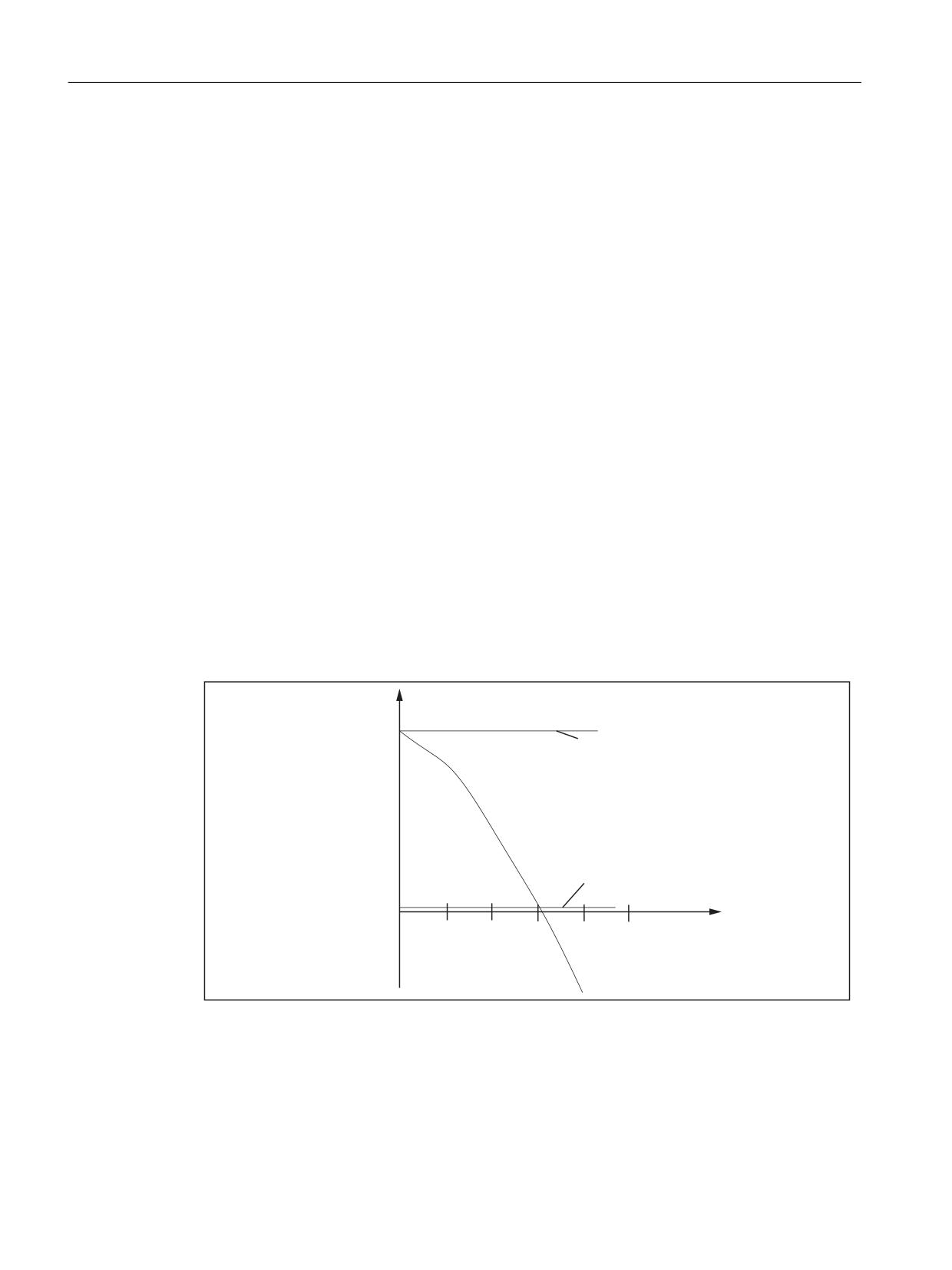
The normalized path is applied as an input quantity: $AC_PATHN.

0: At block start

1: at block end

Variation quantity $AC_OVR must be controlled as a function of $AC_PATHN according to a 3rd

order polynomial. The override must be reduced from 100 to 1% during the motion.

2YHUULGH

$&B295

8SSHU OLPLW

/RZHU OLPLW

3DWK SDUDPHWHUV

$&B3$7+1

Figure 5-3

Regulate velocity continuously

Polynomial 2:

Lower limit: 1

Hi limit: 100

a₀: 100

Synchronized actions

138

Function Manual, 10/2020, 6FC5397-5BP40-6BA4

Examples

5.5 Store execution times in R parameters

: -100

a₂: -100

a₃: not used

With these values, the polynomial definition is as follows:

FCTDEF(2, 1, 100, 100, -100, -100)

; Activation of the variable override as a function of the path:

ID= 1 DO SYNFCT (2, $AC_OVR, $AC_PATHN)

G01 X100 Y100 F1000

5.4

Monitoring a safety clearance between two axes

Task

The axes X1 and X2 operate two independently controlled transport devices used to load and

unload workpieces.

To prevent the axes from colliding, a safety clearance must be maintained between them.

If the safety clearance is violated, then axis X2 is decelerated. This interlock is applied until axis

X1 leaves the safety clearance area again.

If axis X1 continues to move towards axis X2, thereby crossing a closer safety barrier, then it is

traversed into a safe position.

NC language

Comment

ID=1 WHENEVER $AA_IM[X2] -

; Safety barrier

$AA_IM[X1] < 30 DO $AA_OVR[X2]=0

ID=2 EVERY $AA_IM[X2] - $AA_IM[X1]

; Safe position

< 15 DO POS[X1]=0

5.5

Store execution times in R parameters

Task

Store the execution time for part program blocks starting at R parameter 10.

Program

Comment

; The example is

; as follows without symbolic programming:

IDS=1 EVERY $AC_TIMEC==0 DO

; Advance R parameter

$AC_MARKER[0] = $AC_MARKER[0] + 1

; pointer on block change

IDS=2 DO $R[10+$AC_MARKER[0]] =

; Write current time

$AC_TIME

; of block start in each case to R parameter

Synchronized actions

Function Manual, 10/2020, 6FC5397-5BP40-6BA4

139

Examples

5.6 "Centering" with continuous measurement

Program

Comment

; The example is

; as follows with symbolic programming:

DEFINE INDEX AS $AC_MARKER[0]

; Agreements for symbolic

; programming

IDS=1 EVERY $AC_TIMEC==0 DO INDEX =

; Advance R parameter

INDEX + 1

; pointer on block change

IDS=2 DO $R[10+INDEX] = $AC_TIME

; Write current time

; of block start in each case to R parameter

5.6

"Centering" with continuous measurement

Introduction

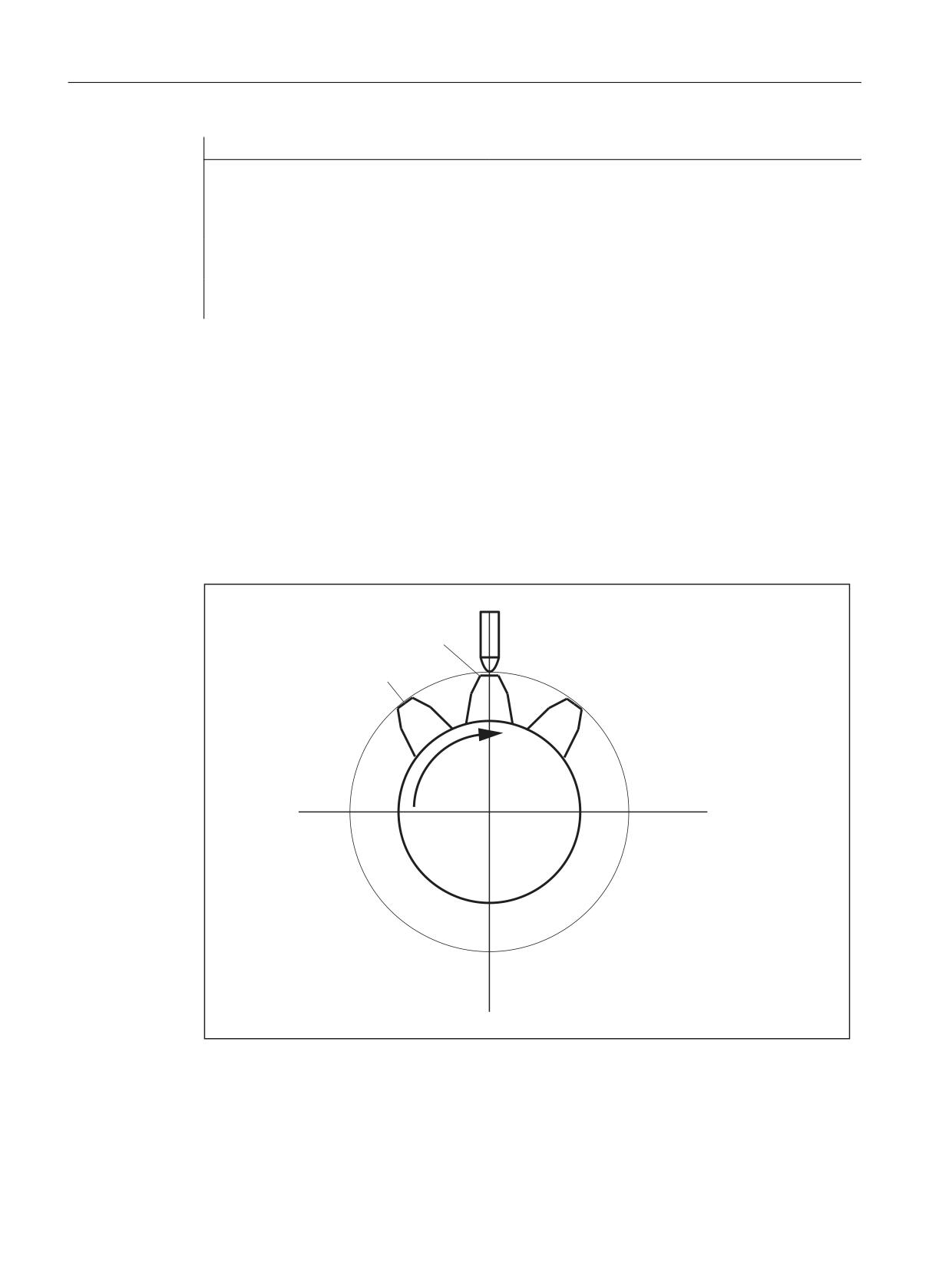
The gaps between gear teeth are measured sequentially. The gap dimension is calculated from

the sum of all gaps and the number of teeth. The center position required to continue machining

is the position of the first measuring point plus 1/2 the average gap size. When measuring, the

speed is selected so that for each interpolation clock cycle a measured value can be reliably

detected.

IDOOLQJ HGJH VWDUW RI JDS

ULVLQJ HGJH HQG RI JDS

3UREH

Figure 5-4

Diagrammatic representation showing how gaps between the gear teeth are measured

Synchronized actions

140

Function Manual, 10/2020, 6FC5397-5BP40-6BA4

Examples

5.6 "Centering" with continuous measurement

%_N_MEAC_MITTEN_MPF

; Measure using rotary axis B (BACH) where the difference is displayed

; between the measured values

;*** Define local user variables ***

N1 DEF INT ZAEHNEZAHL

; Input number of gear teeth

N5 DEF REAL HYS_POS_FLANKE

; Hysteresis positive edge probe

N6 DEF REAL HYS_NEG_FLANKE

; Hysteresis negative edge probe

;*** Define short names for synchronized action markers ***

define M_ZAEHNE as $AC_MARKER[1]

; ID marker for calculation: neg/pos edge per

tooth

define Z_MW as $AC_MARKER[2]

; Read ID counter MW FIFO

define Z_RW as $AC_MARKER[3]

; Calculate ID Counter MW tooth gaps

;*** Input values for ZAHNRADMESSEN ***

N50 ZAEHNEZAHL=26

; Enter number of gear teeth to be measured

N70 HYS_POS_FLANKE = 0.160

; Hysteresis positive edge probe

N80 HYS_NEG_FLANKE = 0.140

; Hysteresis negative edge probe

Start:

*** Assign variables ***

R1=0

; ID2 calculation result for gap dimension

R2=0

; ID2 calculation result addition of all gaps

R3=0

; Content of the first element read

R4=0

; R4 corresponds to a tooth distance

R5=0

; Gap position calculated, final result

R6=1

; Switch-on ID 3 BACH with MOV

R7=1

; Switch-on ID 5 MEAC

M_ZAEHNE=ZAEHNEZAHL*2

; Calculate ID neg./pos. edge per tooth

Z_MW=0

; Read ID counter MW FIFO till the number of

teeth

Z_RW=2

; Calculate ID counter difference of tooth gap

R13=HYS_POS_FLANKE

; Hysteresis in calculation register

R14=HYS_NEG_FLANKE

; Hysteresis in calculation register

;*** Traverse axis, measure, calculate ***

N100 MEAC[BACH]=(0)

; Reset measurement job

; Reset FIFO1[4] variables and ensure a defined measurement trace

N105 $AC_FIFO1[4]=0

; Reset FIFO1

STOPRE

;*** Read out FIFO until the number of teeth reached ***

; If FIFO1 is not empty and all teeth are still not measured, save measured value

from FIFO variable in

; synchronization parameter and increment counter of measured values

ID=1 WHENEVER ($AC_FIFO1[4]>=1) AND (Z_MW<M_ZAEHNE)

DO $AC_PARAM[0+Z_MW]=$AC_FIFO1[0]

Z_MW=Z_MW+1

Synchronized actions

Function Manual, 10/2020, 6FC5397-5BP40-6BA4

141

Examples

5.6 "Centering" with continuous measurement

; if 2 measured values are present, start calculation, calculate ONLY gap dimension

; and gap sum, increment calculation value counter by 2

ID=2 WHENEVER (Z_MW>=Z_RW) AND (Z_RW<M_ZAEHNE)

DO $R1=($AC_PARAM[-1+Z_RW]-$R13)-($AC_PARAM[-2+Z_RW]-$R14)

Z_RW=Z_RW+2 $R2=

$R2+$R1

;*** Switch-on the axis BACH as endless rotating rotary axis with MOV ***

WAITP(BACH)

; Switch on

ID=3 EVERY $R6==1 DO MOV[BACH]=1 FA[BACH]=1000

; Switch off

ID=4 EVERY $R6==0 and ($AA_STAT[BACH]==1) DO MOV[BACH]=0

; Measure sequentially, store in FIFO 1, MT2 neg, MT2 pos edge;the distance between

two teeth is measured

;falling edge-...-rising edge, probe 2

N310 ID=5 WHEN $R7==1 DO MEAC[BACH]=(2, 1, -2, 2)

; Cancel measurement

N320 ID=6 WHEN (Z_MW>=M_ZAEHNE) DO MEAC[BACH]=(0)

M00

STOPRE

;*** Fetch FIFO values and save***

; Content of the first element read

; Reset FIFO1[4] variables and ensure a

; defined measurement trace for the next measuring job

N400 R3=$AC_PARAM[0]

N500 $AC_FIFO1[4]=0

;*** Calculate difference between the individual teeth ***

; R4 corresponds to an average tooth distance

; division "/1000" removed in later SW versions

N510 R4=R2/(ZAEHNEZAHL)/1000

;*** Calculate center position ***

N520 R3=R3/1000

; First measurement position converted to de-

gree

N530 R3=R3 MOD 360

; first measurement point modulo

N540 R5=(R3-R14)+(R4/2)

; Calculate gap position

M00

STOPRE

R6=0

; Deactivate axis rotation from BACH

GOTOB START

M30

Synchronized actions

142

Function Manual, 10/2020, 6FC5397-5BP40-6BA4

Examples

5.7 Axis couplings via synchronized actions

5.7

Axis couplings via synchronized actions

5.7.1

Coupling to leading axis

Task assignment

A cyclic curve table is defined by means of polynomial segments. Controlled by means of

arithmetic variables, the movement of the master axis and the coupling process between master

and slave (following) axes is activated/deactivated.

%_N_KOP_SINUS_MPF

N5 R1=1

; ID 1, 2 activate/deactivate coupling: LEADON

(CACB, BACH)

N6 R2=1

; ID 3, 4 Move leading axis on/off: MOV BACH

N7 R5=36000

; BACH Feedrate/min

N8 STOPRE

;*** Define periodic table No. 4 through polynomial segments ***

N10 CTABDEF (YGEO,XGEO,4,1)

N16 G1 F1200 XGEO=0.000 YGEO=0.000

; Go to basic position

N17 POLY PO[XGEO]=(79,944.30.420,00.210) PO[YGEO]=(24,634.00.871,-9,670)

N18 PO[XGEO]=(116.059,0.749,-0.656) PO[YGEO]=(22.429,-5.201,0.345)

N19 PO[XGEO]=(243.941,-17.234,11.489) PO[YGEO]=(-22.429,-58.844,39.229)

N20 PO[XGEO]=(280.056,1.220,-0.656) PO[YGEO]=(-24.634,4.165,0.345)

N21 PO[XGEO]=(360.000,-4.050,0.210) PO[YGEO]=(0.000,28.139,-9.670)

N22 CTABEND

;

*** End of table definition ***

; Travel axis leading axis and coupled axis in quick motion in basic position

N80 G0 BACH=0 CACH=0

; Channel axis names

N50 LEADOF(CACH,BACH)

; existing coupling OFF

N235 ;*** Switch-on the coupling movement for the axis CACH ***

N240 WAITP(CACH)

; Synchronize axis to channel

N245 ID=1 EVERY $R1==1 DO LEA-

; Coupling via table 4

DON(CACH, BACH, 4)

N250 ID=2 EVERY $R1==0 DO LEA-

; Deactivate coupling

DOF(CACH, BACH)

N265 WAITP(BACH)

Synchronized actions

Function Manual, 10/2020, 6FC5397-5BP40-6BA4

143

Examples

5.7 Axis couplings via synchronized actions

N270 ID=3 EVERY $R2==1 DO

; Rotate leading axis with feedrate endlessly

MOV[BACH]=1 FA[BACH]=R5

in R5

N275 ID=4 EVERY $R2==0 DO

; Stop leading axis

MOV[BACH]=0

N280 M00

N285 STOPRE

N290 R1=0

; Disable coupling condition

N295 R2=0

; Disable condition for rotating leading axis

N300 R5=180

; New feedrate for BACH

N305 M30

5.7.2

Non-circular grinding via master value coupling

Task assignment

A non-circular workpiece that is rotating on axis CACH must be machined by grinding. The

distance between the grinding wheel and workpiece is controlled by axis XACH and depends on

the angle of rotation of the workpiece. The interrelationship between angles of rotation and

assigned movements is defined in curve table 2. The workpiece must move at velocities that are

determined by the workpiece contour defined in curve table 1.

Solution

CACH is designated as the leading axis in a master value coupling. It controls:

• via table 2 the compensatory movement of the axis XACH

• via table 1 the "software axis" CASW.

The axis override of axis CACH is determined by the actual values of axis CASW, thus providing

the required contour-dependent velocity of axis CACH.

Synchronized actions

144

Function Manual, 10/2020, 6FC5397-5BP40-6BA4

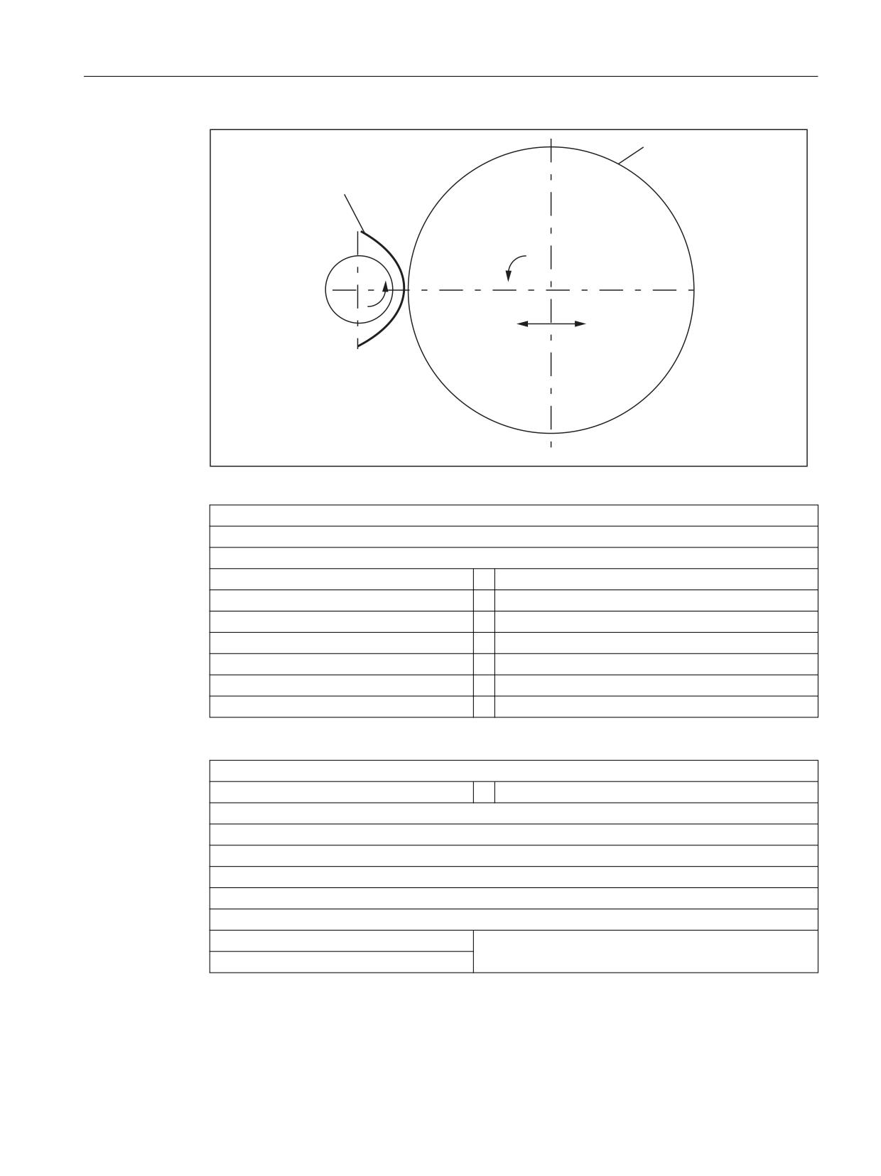
Examples

5.7 Axis couplings via synchronized actions

*ULQGLQJ GLVF

6HFWLRQ RI

:RUNSLHFH FRQWRXU

&$&

;$&+

Figure 5-5

Diagrammatic representation of non-circular contour grinding

%_N_CURV_TABS_SPF

PROC CURV_TABS

N160 ; *** Define table 1 override ***

N165 CTABDEF(CASW,CACH,1.1)

;

Table 1 periodic

N170 CACH=0 CASW=10

N175 CACH=90 CASW=10

N180 CACH=180 CASW=100

N185 CACH=350 CASW=10

N190 CACH=359.999 CASW=10

N195 CTABEND

N160 ; *** Define table 2 linear compensatory movement of XACH ***

CTABDEF(YGEO,XGEO,2.1)

;

Table 2 periodic

N16 XGEO=0.000 YGEO=0.000

N16 XGEO=0.001 YGEO=0.000

N17 POLY PO[XGEO]=(116.000,0.024,0.012) PO[YGEO]=(4.251,0.067,-0.828)

N18 PO[XGEO]=(244.000,0.072,-0.048) PO[YGEO]=(4.251,-2.937)

N19 PO[XGEO]=(359.999,-0.060,0.012) PO[YGEO]=(0.000,-2.415,0.828)

N16 XGEO=360.000 YGEO=0.000

N20 CTABEND

M17

%_N_UNRUND_MPF

; Coupling group for a non-circular machining

; XACH is the infeed axis of the grinding disk

Synchronized actions

Function Manual, 10/2020, 6FC5397-5BP40-6BA4

145

Examples

5.7 Axis couplings via synchronized actions

; CACH is the workpiece axis as rotary axis and master value axis

; Application: Grind non-circular contours

; Table 1 maps the override for axis CACH as function of the position of CACH

; Overlay of the XGEO axis with handwheel infeed for scratching

N100 DRFOF

;

deselect handwheel overlay

N200 MSG(Select "DRF, (Handwheel 1 active) and Select INKREMENT.== Handwheel overlay AKTIV")

N300 M00

N500 MSG()

;

Reset message

N600 R2=1

;

LEADON Table 2, Activate with ID=3/4 CACH to XACH

N700 R3=1

;

LEADON Table 1, Activate with ID=5/6 CACH to CASW,

override

N800 R4=1

;

Endless rotating axis CACH, start with ID=7/8

N900 R5=36000

;

FA[CACH] Endless rotating rotary axis speed

N1100 STOPRE

N1200

;

*** Set axis and leading axis to FA ***

;

Move Axis, master axis and following axis

;

to the initial position

N1300 G0 XGEO=0 CASW=10 CACH=0

N1400 LEADOF(XACH,CACH)

;

Coupling AUS XACH compensatory movement

N1500 LEADOF(CASW,CACH)

;

Coupling AUS CASW override table

N1600 CURV_TABS

;

Sub-program with definition of the tables

N1700

;

*** On-off switch of the LEADON compensatory move-

ment XACH ***

N1800 WAITP(XGEO)

;

Synchronize axis to channel

N1900 ID=3 EVERY $R2==1 DO LEA-

DON(XACH,CACH,2)

N2000 ID=4 EVERY $R2==0 DO LEA-

DOF(XACH,CACH)

N2100

;

*** On-off switch of the LEADON CASW

;

override table ***

N2200 WAITP(CASW)

N2300 ID=5 EVERY $R3==1 DO LEA-

;

CTAB Coupling ON leading axis CACH

DON(CASW,CACH,1)

N2400 ID=6 EVERY $R3==0 DO LEA-

;

CTAB Coupling OFF leading axis CACH

DOF(CASW,CACH)

Synchronized actions

146

Function Manual, 10/2020, 6FC5397-5BP40-6BA4

Examples

5.7 Axis couplings via synchronized actions

N2500

;

*** Control override of the CACH from position

;

CASW with ID 10 ***

N2700 ID=11 DO $$AA_OVR[CACH]=

;

Assign "axis position" CASW to OVR CACH

$AA_IM[CASW]

N2900 WAITP(CACH)

N3000 ID=7 EVERY $R4==1 DO

;

Start as endless rotating rotary axis

MOV[CACH]=1 FA[CACH]=R5

N3100 ID=8 EVERY $R4==0 DO

;

Stop as endless rotating rotary axis

MOV[CACH]=0

N3200 STOPRE

N3300 R90=$AA_COUP_ACT[CASW]

;

State of the coupling for CASW for checking

N3400 MSG("Override table CASW activated with LEADON "<<R90<<", further ENDE with NC-START")

N3500 M00

;

*** NC HALT ***

N3600 MSG()

N3700 STOPRE

;

Preprocessing stop

N3800 R1=0

;

Stop with ID=2 CASW axis as

;

endless rotating rotary axis

N3900 R2=0

;

LEADOF with ID=6 FA XACH

;

and leading axis CACH

N4000 R3=0

;

LEADOF TAB1 CASW with ID=7/8 CACH

;

to CASW override table

N4100 R4=0

;

Stop axis as endless rotating rotary axis

;

, ID=4 CACH

N4200 M30

Expansion options

The example above can be expanded by the following components:

• Introduction of a Z axis to move the grinding wheel or workpiece from one non-circular

operation to the next on the same shaft (cam shaft).

• Table switchovers, if the cams for inlet and outlet have diferent contours.

ID = ... <Condition> DO LEADOF(XACH, CACH) LEADON(XACH, CACH, <new

table number>)

• Dressing of grinding wheel by means of online tool offset acc. to Subsection "Online tool

offset FTOC".

Synchronized actions

Function Manual, 10/2020, 6FC5397-5BP40-6BA4

147

Examples

5.7 Axis couplings via synchronized actions

5.7.3

On-the-fly parting

Task assignment

An extruded material which passes continuously through the operating area of a cutting tool

must be cut into parts of equal length.

X axis: Axis in which the extruded material moves, WCS

X1 axis: Machine axis of the extruded material, MCS

Y axis: Axis in which the cutting tool "tracks" the extruded material

It is assumed that the infeed and control of the cutting tool are controlled via the PLC. The signals

at the PLC interface can be evaluated to determine whether the extruded material and cutting

tool are synchronized.

Actions

Activate coupling, LEADON

Deactivate coupling, LEADOF

Set actual values, PRESETON

Program code

Comment

%_N_SCHERE1_MPF

;$PATH=/_N_WKS_DIR/_N_DEMOFBE_WPD

N100 R3=1500

; Length of a part to be cut off

N200 R2=100000 R13=R2/300

N300 R4=100000

N400 R6=30

; Start position Y axis

N500 R1=1

; Start condition for conveyor axis

N600 LEADOF(Y,X)

; Delete any existing coupling

N700 CTABDEF(Y,X,1,0)

; Table definition

N800 X=30 Y=30

; Value pairs

N900 X=R13 Y=R13

N1000 X=2*R13 Y=30

N1100 CTABEND

; End of table definition

N1200 PRESETON(X1,0)

; Preset offset at the beginning

N1300 Y=R6 G0

; Start position Y axis

; The axis is a linear axis

N1400 ID=1 EVERY $AA_IW[X]>$R3 DO PRESETON(X1,0)

; Preset offset after length R3, PRESE-

TON must only be executed with WHEN

and EVERY

; New start after parting

N1500 WAITP(Y)

N1800 ID=6 EVERY $AA_IM[X]<10 DO LEADON(Y,X,1)

; For X < 10, couple Y to X via table 1

N1900 ID=10 EVERY $AA_IM[X]>$R3-30 DO LEADOF(Y,X)

; > 30 before traversed parting dis-

tance, deactivate coupling

N2000 WAITP(X)

Synchronized actions

148

Function Manual, 10/2020, 6FC5397-5BP40-6BA4

Examples

5.8 Technology cycles position spindle

Program code

Comment

N2100 ID=7 WHEN $R1==1 DO MOV[X]=1 FA[X]=$R4

; Set extruded material axis continuous-

ly in motion

N2200 M30

5.8

Technology cycles position spindle

Application

Interacting with the PLC program, the spindle which initiates a tool change should be:

• Traversed to an initial position,

• Positioned at a specific point at which the tool to be inserted is located.

See Section "Starting command axes" and Section "Control via PLC".

Coordination

The PLC and NCK are coordinated by means of the common data that are provided in SW version

4 and later (see Section "List of system variables relevant to synchronized actions")

• $A_DBB[0]: Go to basic position 1,

• $A_DBB[1]: Go to target position 1,

• $A_DBW[1]: Value to be positioned +/- , PLC calculates the shortest route.

Synchronized actions

%_N_MAIN_MPF

IDS=1 EVERY $A_DBB[0]==1 DO NULL_POS

; When $A_DBB[0] set by PLC, go

to basic position.

IDS=2 EVERY $A_DBB[1]==1 DO ZIEL_POS

; When $A_DBB[1] set by PLC, po-

sition spindle to the value stor-

ed in$A_DBW[1].

Technology cycle NULL_POS

%_N_NULL_POS_SPF

PROC NULL_POS

SPOS=0

; Put drive for the tool change into basic posi-

tion.

$A_DBB[0]=0

; Basic position executed in NC.

Synchronized actions

Function Manual, 10/2020, 6FC5397-5BP40-6BA4

149

Examples

5.9 Synchronized actions in the TC/MC area

Technology cycle ZIEL_POS

%_N_ZIEL_POS_SPF

PROC ZIEL_POS

SPOS=IC($A_DBW[1])

; Traverse spindle to position value that has been

stored in $A_DBW[1] by the PLC, incremental dimen-

sion

$A_DBB[1]=0

; Target positions executed in NC.

5.9

Synchronized actions in the TC/MC area

Introduction

The following figure shows the schematic structure of a tool-changing cycle.

= UHOHDVHG

0DJD]LQH 3RVLWLRQLQJ

5HWXUQ WRRO

)HWFK 722/

/HYHO WRRO SRFNHWV

:3<

:3;

= FODPSHG

,QWHUPHGLDWH SRLQW

=3 <

FDQ EH URXQGHG

=3 ;

93<

93;

6WDUWLQJ SRLQW

93;

6WDUWLQJ SRLQW

= FODPSHG

= UHOHDVHG

;

Figure 5-6

Schematic sequence for tool-changing cycle

Synchronized actions

150

Function Manual, 10/2020, 6FC5397-5BP40-6BA4

Examples

5.9 Synchronized actions in the TC/MC area

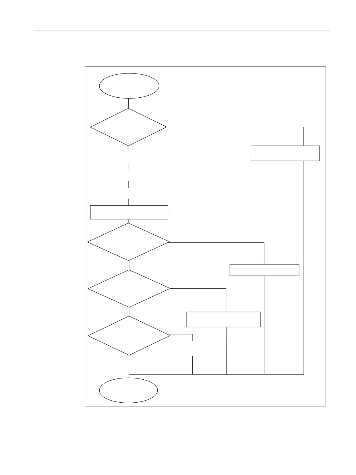
Flow diagram

6WDUW

7RRO FKDQJH F\FOH LQ

03)

<HV

%ORFN VHDUFK DFWLYH"

,I 3B6($5&+ *272)

7RRO FKDQJH 0

3RVLWLRQ VSLQGOHV RYHU EORFN OLPLWV

' $FWLYDWH WRRO RIIVHW

6326$ RU 6326$>Q@

5HDG SUHVHW 7 QXPEHU

*(76(/7>@ RU *(76(/7> Q@

5HDG 7 QXPEHU IURP VSLQGOH

7RRO6SLQGOH

7&B033 >

&KDQJH WRRO

3UHVHOHFWHG WRRO LQ 63"

<HV

,I :=6SLQGOH

:=6HOHFWLRQ

*272)

' $FWLYDWH WRRO RIIVHW

3UHVHOHFWHG 7 1R

<HV

,I 7RROFRGH

*272)

5HWXUQ WRRO

' 'HDFWLYDWH WRRO RIIVHW

<HV

1R WRRO LQ VSLQGOH"

,I 7RRO6SLQGOH

*272)

)HWFK 722/

' $FWLYDWH WRRO RIIVHW

VW 5HWXUQ WRRO QG )HWFK WRRO

' $FWLYDWH WRRO RIIVHW

(QG

Figure 5-7

Flow diagram for tool changing cycle

Synchronized actions

Function Manual, 10/2020, 6FC5397-5BP40-6BA4

151

Examples

5.9 Synchronized actions in the TC/MC area

NC program

Comment

%_N_WZW_SPF

;$PATH=/_N_SPF_DIR

N10 DEF INT WZVorwahl,WZSpindel

;Marker on = 1 when MagAxis traversed

N15 WHEN $AC_PATHN<10 DO $AC_MARKER[0]=0 $AC_MARKER[1]=0

$AC_MARKER[2]=0

N20 ID=3 WHENEVER $A_IN[9]==TRUE DO $AC_MARKER[1]=1

N25 ID=4 WHENEVER $A_IN[10]==TRUE DO $AC_MARKER[2]=1

;Marker on = 1 when MagAxis traversed

N30 IF $P_SEARCH GOTOF wzw_vorlauf

;Block preprocessing active ? ->

N35 SPOSA=0 D0

N40 GETSELT(WZVorwahl)

;Read preselected T no.

N45 WZSpindel=$TC_MPP6[9998,1]

;Read tool in spindle

N50 M06

N55 IF WZSpindel==WZVorwahl GOTOF wz_in_spindel IF WZVor-

wahl==0 GOTOF ablegen1 IF WZSpindel==0 GOTOF holen1

;*** Fetch and store tool***

ablegen1holen1:

N65 WHENEVER $AA_VACTM[C2]<>0 DO $AC_MARKER[1]=1

;when MagAxis travels Marker = 1

N70 G01 G40 G53 G64 G90 X=Magazin1VPX Y=Magazin1VPY Z=Maga-

zin1ZGespannt F70000 M=QU(120) M=QU(123) M=QU(9)

N75 WHENEVER $AA_STAT[S1]<>4 DO $AC_OVR=0

;Spindle in position

N80 WHENEVER $AA_VACTM[C2]<>0 DO $AC_MARKER[1]=1

;Query MagAxis travel

N85 WHENEVER $AC_MARKER[1]==0 DO $AC_OVR=0

;Override=0 when axis not traversed

N90 WHENEVER $AA_STAT[C2]<>4 DO $AC_OVR=0

;Override=0 when MagAxis

not in position fine

N95 WHENEVER $AA_DTEB[C2]>0 DO $AC_OVR=0

;Override=0 when distance-to-go MagAx-

is > 0

N100 G53 G64 X=Magazin1ZP1X Y=Magazin1ZP1Y F60000

N105 G53 G64 X=Magazin1WPX Y=Magazin1WPY F60000

N110 M20

;Release tool

N115 G53 G64 Z=MR_Magazin1ZGeloest F40000

N120 WHENEVER $AA_VACTM[C2]<>0 DO $AC_MARKER[2]=1;

N125 WHENEVER $AC_MARKER[2]==0 DO $AC_OVR=0

N130 WHENEVER $AA_STAT[C2]<>4 DO $AC_OVR=0

N135 WHENEVER $AA_DTEB[C2]>0 DO $AC_OVR=0

N140 G53 G64 Z=Magazin1ZGespannt F40000

N145 M18

;Clamp tool

N150 WHEN $AC_PATHN<10 DO M=QU(150) M=QU(121)

;Condition always fulfilled

N155 G53 G64 X=Magazin1VPX Y=Magazin1VPY F60000 D1 M17

Synchronized actions

152

Function Manual, 10/2020, 6FC5397-5BP40-6BA4

Examples

5.9 Synchronized actions in the TC/MC area

NC program

Comment

;*** Store tool***

ablegen1:

N160 WHENEVER $AA_VACTM[C2]<>0 DO $AC_MARKER[1]=1

N165 G01 G40 G53 G64 G90 X=Magazin1VPX Y=Magazin1VPY Z=Maga-

zin1ZGespannt F70000 M=QU(120) M=QU(123) M=QU(9)

N170 WHENEVER $AA_STAT[S1]<>4 DO $AC_OVR=0

N175 WHENEVER $AA_VACTM[C2]<>0 DO $AC_MARKER[1]=1

N180 WHENEVER $AC_MARKER[1]==0 DO $AC_OVR=0

N185 WHENEVER $AA_STAT[C2]<>4 DO $AC_OVR=0

N190 WHENEVER $AA_DTEB[C2]>0 DO $AC_OVR=0

N195 G53 G64 X=Magazin1ZP1X Y=Magazin1ZP1Y F60000

N200 G53 G64 X=Magazin1WPX Y=Magazin1WPY F60000

N205 M20

;Release tool

N210 G53 G64 Z=Magazin1ZGeloest F40000

N215 G53 G64 X=Magazin1VPX Y=Magazin1VPY F60000 M=QU(150)

M=QU(121) D0 M17

;*** Fetch tool***

holen1:

N220 WHENEVER $AA_VACTM[C2]<>0 DO $AC_MARKER[2]=1

N225 G01 G40 G53 G64 G90 X=Magazin1VPX Y=Magazin1VPY Z=Maga-

zin1ZGeloest F70000 M=QU(120) M=QU(123) M=QU(9)

N230 G53 G64 X=Magazin1WPX Y=Magazin1WPY F60000

N235 WHENEVER $AA_STAT[S1]<>4 DO $AC_OVR=0

N240 WHENEVER $AA_VACTM[C2]<>0 DO $AC_MARKER[2]=1

N245 WHENEVER $AC_MARKER[2]==0 DO $AC_OVR=0

N250 WHENEVER $AA_STAT[C2]<>4 DO $AC_OVR=0

N255 WHENEVER $AA_DTEB[C2]>0 DO $AC_OVR=0

N260 G53 G64 Z=Magazin1ZGespannt F40000

N265 M18

;Clamp tool

N270 G53 G64 X=Magazin1VPX Y=Magazin1VPY F60000 M=QU(150)

M=QU(121) D1 M17

;***Tool in spindle***

wz_in_spindle:

N275 M=QU(121) D1 M17

;***Block preprocessing***

wzw_feed:

N280 STOPRE

N285 D0

N290 M06

N295 D1 M17

Synchronized actions

Function Manual, 10/2020, 6FC5397-5BP40-6BA4

153

Data lists

6.1

Machine data

6.1.1

General machine data

Number

Identifier: $MN_

Description

11110

AUXFU_GROUP_SPEC

Auxiliary function group specification

11500

PREVENT_SYNACT_LOCK

Protected synchronized actions

18860

MM_MAINTENANCE_MON

Activate recording of maintenance data

6.1.2

Channelspecific machine data

Number

Identifier: $MC_

Description

21240

PREVENT_SYNACT_LOCK_CHAN

Protected synchronized actions for channel

28250

MM_NUM_SYNC_ELEMENTS

Number of elements for expressions in synchronized

actions

28252

MM_NUM_FCTDEF_ELEMENTS

Number of FCTDEF elements

28254

MM_NUM_AC_PARAM

Number of $AC_PARAM parameters

28255

MM_BUFFERED_AC_PARAM

Memory location of $AC_PARAM

28256

MM_NUM_AC_MARKER

Number of $AC_MARKER markers

28257

MM_BUFFERED_AC_MARKER

Memory location of $AC_MARKER

28258

MM_NUM_AC_TIMER

Number of $AC_TIMER time variables

28260

NUM_AC_FIFO

Number of $AC_FIFO1, $AC_FIFO2, ... variables

28262

START_AC_FIFO

Store FIFO variables from R parameter

28264

LEN_AC_FIFO

Length of $AC_FIFO ... FIFO variables

28266

MODE_AC_FIFO

FIFO processing mode

6.1.3

Axis-specific machine data

Number

Identifier: $MA_

Description

30450

IS_CONCURRENT_POS_AX

Concurrent positioning axis

32060

POS_AX_VELO

Initial setting for positioning axis velocity

32070

CORR_VELO

Axial velocity for handwheel, ext. WO (work offset),

cont. dressing, clearance control

Synchronized actions

Function Manual, 10/2020, 6FC5397-5BP40-6BA4

155

Data lists

6.2 Setting data

Number

Identifier: $MA_

Description

32074

FRAME_OR_CORRPOS_NOTALLOWED

Effectiveness of frames and tool length offset

32920

AC_FILTER_TIME

Filter smoothing time constant for Adaptive Control

33060

MAINTENANCE_DATA

Configuration, recording maintenance data

36750

AA_OFF_MODE

Effect of value assignment for axial override with

synchronized actions

37200

COUPLE_POS_TOL_COARSE

Threshold value for "Coarse synchronism"

37210

COUPLE_POS_TOL_FINE

Threshold value for "Fine synchronism"

6.2

Setting data

6.2.1

Axis/spindle-specific setting data

Number

Identifier: $SA_

Description

43300

ASSIGN_FEED_PER_REV_SOURCE

Rotational feedrate for positioning axes/spindles

43350

AA_OFF_LIMIT

Upper limit of offset value for $AA_OFF clearance con-

trol

43400

WORKAREA_PLUS_ENABLE

Working area limitation in pos. direction

Synchronized actions

156

Function Manual, 10/2020, 6FC5397-5BP40-6BA4

Preface

Introduction

Fundamental safety

instructions

SINUMERIK

Installation and activation

of loadable compile cycles

SINUMERIK 840D sl

Technologies

Simulation of compile

cycles (only HMI Advanced)

Clearance control (CLC/

CLCX)

Function Manual

Speed/torque coupling,

master-slave

Transformation package

handling

MCS coupling

Continue machining

(retrace support)

Cycle-independent path-

synchronous switching

signal output (HSLC)

Axis pair collision protection

Punching and nibbling

Appendix

Valid for

control system

SINUMERIK 840D sl / 840DE sl

CNC software Version 4.94

10/2020

6FC5397-8GP40-0BA1

Table of contents

Preface

Introduction

1.1

About this documentation

Fundamental safety instructions

2.1

General safety instructions

2.2

Warranty and liability for application examples

2.3

Security information

Installation and activation of loadable compile cycles

3.1

Loading compile cycles

3.1.1

Loading a compile cycle with SINUMERIK Operate

3.1.2

Loading a compile cycle with HMI Advanced

3.1.3

Loading a compile cycle from an external computer with WinSCP

3.2

Interface version compatibility

3.3

Software version of a compile cycle

3.4

Activating the technological functions in the NC

3.5

Function-specific startup

3.6

Creating alarm texts

3.6.1

Creating alarm texts with SINUMERIK Operate

3.7

Upgrading a compile cycle

3.8

Deleting a compile cycle

3.9

Data lists

3.9.1

Machine data

3.9.1.1

NC-specific machine data

Simulation of compile cycles (only HMI Advanced)

4.1

Brief description

4.1.1

Function

4.2

OEM transformations

Clearance control (CLC/CLCX)

5.1

Brief description

5.1.1

Function description

5.2

Clearance control

5.2.1

POS mode

5.2.1.1

Overview

5.2.1.2

POS mode

5.2.2

GAIN mode

Technologies

Function Manual, 10/2020, 6FC5397-8GP40-0BA1

Table of contents

5.2.2.1

Control dynamics - GAIN mode

5.2.3

Dead times in the clearance control

5.2.4

Optimizing the control behavior

5.3

Technological features of clearance control

5.4

Sensor collision monitoring

5.5

Startup

5.5.1

Setup steps

5.5.2

Activating the technological function

5.5.3

Configuring the memory

5.5.4

Sensor input and sensor signals

5.5.4.1

Setting up the analog sensor input

5.5.4.2

Parameterizing the input signals

5.5.4.3

Simulation of the sensor signals

5.5.4.4

Linearizing the signal of the clearance sensor

5.5.4.5

Compensation of the time delay of the sensor

5.5.5

Parameter settings for clearance control

5.5.6

Configuration of the basic MD of CLCX

5.5.7

Definition of the real-time variables for synchronized actions

5.6

Programming

5.6.1

Activating and deactivating clearance control (CLC)

5.6.2

NC commands and Synact variables

5.6.3

Synact variables for diagnostics

5.6.4

Available technology commands

5.6.5

Diagnosis of the CLCX state

5.7

3D clearance control

5.7.1

3D clearance control - overview

5.7.2

3D control direction

5.7.3

Parameterization of the programmable control direction

5.7.4

3D clearance control and 5-axis transformation

5.8

Multiple CLCX instances in different channels

5.8.1

Multiple CLCX instances in one channel

5.8.2

Macros for operating and monitoring multiple instances in one channel

5.8.3

Programming several instances within one channel

5.8.4

Additional voltage/clearance characteristics

5.9

Function-specific display data

5.9.1

Channel-specific GUD variables

5.10

Function-specific alarm texts

5.11

Supplementary conditions

5.11.1

I/O modules

5.11.1.1

External smoothing filters

5.11.2

Function-specific supplementary conditions

5.12

Data lists

5.12.1

Machine data

5.12.1.1

NC-specific machine data

5.12.1.2

Channelspecific machine data

5.12.1.3

Axis/spindlespecific machine data

Technologies

Function Manual, 10/2020, 6FC5397-8GP40-0BA1

Table of contents

Speed/torque coupling, master-slave

6.1

Brief description

6.2

Coupling diagram

6.3

Configuring a coupling

6.4

Torque compensatory controller

6.5

Tension torque

6.6

Closing/opening a coupling

6.7

Response on activation/deactivation

6.8

Supplementary conditions

101

6.8.1

Functional boundary conditions

101

6.8.2

Axial NC/PLC interface signals

103

6.8.3

Interaction with other functions

104

6.9

Examples

109

6.9.1

Master-slave coupling between AX1=Master and AX2=Slave

109

6.9.2

Close coupling via the PLC

110

6.9.3

Close/separate coupling via part program

110

6.9.4

Release the mechanical brake

111

6.10

Data lists

112

6.10.1

Machine data

112

6.10.1.1

Axis/spindlespecific machine data

112

6.10.2

System variables

112

Transformation package handling

113

7.1

Brief description

113

7.2

Kinematic transformation

114

7.3

Definition of terms

114

7.3.1

Units and directions

114

7.3.2

Definition of positions and orientations using frames

115

7.3.3

Definition of a joint

116

7.4

Configuration of a kinematic transformation

117

7.4.1

General machine data

117

7.4.2

Parameterization using geometry data

118

7.5

Descriptions of kinematics

130

7.5.1

3-axis kinematics

130

7.5.2

4-axis kinematics

137

7.5.3

5-axis kinematics

143

7.5.4

6-axis kinematics

147

7.5.5

Special kinematics

148

7.6

Tool orientation

152

7.6.1

Orientation programming for 4-axis kinematics

154

7.6.2

Orientation programming for 5-axis kinematics

156

7.7

Singular positions and how they are handled

157

7.8

Call and application of the transformation

157

Technologies

Function Manual, 10/2020, 6FC5397-8GP40-0BA1

Table of contents

7.9

Actual value display

159

7.10

Tool programming

159

7.11

Cartesian PTP travel with handling transformation package

160

7.12

Startup

160

7.12.1

General commissioning

160

7.12.2

Function-specific commissioning

160

7.13

Supplementary conditions

162

7.14

Data lists

163

7.14.1

Machine data

163

7.14.1.1

General machine data

163

7.14.1.2

Channelspecific machine data

164

7.14.1.3

Channel-specific machine data for compile cycles

164

MCS coupling

167

8.1

Brief description

167

8.2

Description of MCS coupling functions

168

8.2.1

Defining coupling pairs

168

8.2.2

Switching the coupling ON/OFF

169

8.2.3

Tolerance window

170

8.2.4

Memory configuration: Block memory

170

8.3

Description of collision protection

170

8.3.1

Defining protection pairs

170

8.3.2

Switching collision protection ON / OFF

171

8.3.3

Configuring example

172

8.4

User-specific configurations

173

8.5

Special operating states

173

8.6

Boundary conditions

174

8.7

Data lists

175

8.7.1

Machine data

175

8.7.1.1

Channelspecific machine data

175

8.7.1.2

Axis/spindlespecific machine data

175

Continue machining (retrace support)

177

9.1

Brief description

177

9.2

Function description

178

9.2.1

Function

178

9.2.2

Definition of terms

180

9.2.3

Functional sequence (principle)

180

9.2.4

Maximum retraceable contour area

184

9.3

Startup

184

9.3.1

Activation

184

9.3.2

Definition of the RESU working plane

185

9.3.3

Memory configuration: Block memory

185

9.3.4

Memory configuration: Heap memory

186

9.3.5

RESU main program memory area

187

Technologies

Function Manual, 10/2020, 6FC5397-8GP40-0BA1

Table of contents

9.3.6

Storage of the RESU subroutines

188

9.3.7

ASUB enable

188

9.3.8

PLC user program

189

9.4

Programming

190

9.4.1

RESU Start/Stop/Reset (CC_PREPRE)

190

9.5

RESU-specific part programs

191

9.5.1

Overview

191

9.5.2

Main program (CC_RESU.MPF)

192

9.5.3

INI program (CC_RESU_INI.SPF)

193

9.5.4

END program (CC_RESU_END.SPF)

195

9.5.5

Retrace support ASUB (CC_RESU_BS_ASUP.SPF)

195

9.5.6

RESU ASUB (CC_RESU_ASUP.SPF)

196

9.6

Retrace support

197

9.6.1

General information

197

9.6.2

Block search with calculation on contour

197

9.6.3

Reposition

198

9.6.4

Temporal conditions concerning NC start

199

9.6.5

Block search from last main block

199

9.7

Function-specific display data

200

9.7.1

Channel-specific GUD variables

200

9.8

Function-specific alarm texts

201

9.9

Boundary conditions

202

9.9.1

Function-specific supplementary conditions

202

9.9.1.1

Continue machining within subprograms

202

9.9.1.2

Continue machining within program loops

202

9.9.1.3

Machining continuation on full circles

203

9.9.1.4

Automatically generated contour elements

203

9.9.2

Supplementary conditions for standard functions

203

9.9.2.1

Axis replacement

203

9.9.2.2

Traversing movements of the channel axes

203

9.9.2.3

Block numbers

204

9.9.2.4

Block search

204

9.9.2.5

Transformations

204

9.9.2.6

Compensations

205

9.9.2.7

Frames

205

9.9.2.8

Tool offsets

206

9.10

Data lists

206

9.10.1

Machine data

206

9.10.1.1

General machine data

206

9.10.1.2

Channelspecific machine data

206

Cycle-independent path-synchronous switching signal output (HSLC)

209

10.1

Brief description

209

10.2

Functional description

210

10.2.1

General information

210

10.2.2

Calculating the switching positions

210

10.2.2.1

Block-related switching signal output

210

10.2.2.2

Path length-related switching signal output

211

Technologies

Function Manual, 10/2020, 6FC5397-8GP40-0BA1

Table of contents

10.2.3

Calculating the switching instants

212

10.2.4

Switching frequency and switching position distance

212

10.2.5

Approaching switching position

214

10.2.6

Programmed switching position offset

214

10.2.7

Response to part program interruption

215

10.3

Startup

215

10.3.1

Activation

215

10.3.2

Memory configuration

215

10.3.3

Parameterizing the digital on-board outputs

216

10.3.4

Parameterizing the switching signal

216

10.3.5

Parameterization of the geometry axes

217

10.4

Programming

217

10.4.1

Activating the block-related switching signal output (CC_FASTON)

217

10.4.2

Activating the path length-related switching signal output (CC_FASTON_CONT)

218

10.4.3

Deactivation (CC_FASTOFF)

219

10.5

Function-specific alarm texts

220

10.6

Supplementary conditions

220

10.6.1

Block search

220

10.6.2

Transformations

221

10.6.3

Transformations

222

10.6.4

Compensations

222

10.6.5

Tool radius compensation (TRC)

222

10.6.6

Continuous-path mode

222

10.6.7

Software cams

223

10.7

Data lists

223

10.7.1

Machine data

223

10.7.1.1

General machine data

223

10.7.1.2

Channelspecific machine data

223

Axis pair collision protection

225

11.1

Brief description

225

11.2

Functional description

225

11.3

Commissioning

226

11.3.1

Enabling the technology function (option)

226

11.3.2

Activating the technology function

227

11.3.3

Activating the supplementary functions

227

11.3.4

Definition of an axis pair

227

11.3.5

Retraction direction

228

11.3.6

Offset for the machine coordinate systems

228

11.3.7

Protection window

229

11.3.8

Orientation

230

11.3.9

Protection window extension

230

11.3.10

Activating the protection function

231

11.3.11

Axis-specific acceleration

232

11.3.12

Monitoring status (GUD)

232

11.3.13

PLC interface: Axis-specific braking operations

233

11.3.14

PLC interface: Axis pair-specific activation of the protection function

234

11.4

Boundary conditions

234

Technologies

Function Manual, 10/2020, 6FC5397-8GP40-0BA1

Table of contents

11.4.1

Axes

234

11.4.2

Axis container

235

11.4.3

Link axes

236

11.4.4

Interpolatory couplings

236

11.5

Examples

237

11.5.1

Collision protection

237

11.5.2

Collision protection and distance limiter

238

11.6

Data lists

240

11.6.1

Option data

240

11.6.2

Machine data

240

11.6.2.1

NC-specific machine data

240

11.6.2.2

Axis/Spindle-specific machine data

240

11.6.3

User data

240

11.6.3.1

Global user data (GUD)

240

Punching and nibbling

241

12.1

Brief Description

241

12.2

Stroke control

241

12.2.1

General information

241

12.2.2

High-speed signals

242

12.2.3

Criteria for stroke initiation

243

12.2.4

Axis start after punching

245

12.2.5

PLC signals specific to punching and nibbling

246

12.2.6

Punching and nibbling-specific reactions to standard PLC signals

247

12.2.7

Signal monitoring

247

12.3

Activation and deactivation

247

12.3.1

Language commands

247

12.3.2

Functional expansions

252

12.3.3

Compatibility with earlier systems

255

12.4

Automatic path segmentation

257

12.4.1

General information

257

12.4.2

Operating characteristics with path axes

258

12.4.3

Response in connection with single axes

263

12.5

Rotatable tool

267

12.5.1

General information

267

12.5.2

Coupled motion of punch and die

268

12.5.3

Tangential control

269

12.6

Protection zones

272

12.7

Supplementary conditions

272

12.8

Examples

273

12.8.1

Examples of defined start of nibbling operation

273

12.9

Data lists

278

12.9.1

Machine data

278

12.9.1.1

General machine data

278

12.9.1.2

Channelspecific machine data

278

12.9.2

Setting data

278

12.9.2.1

Channelspecific setting data

278

Technologies

Function Manual, 10/2020, 6FC5397-8GP40-0BA1

Introduction

1.1

About this documentation

This documentation is part of the documentation category of SINUMERIK Function Manuals.

SINUMERIK Function Manuals

The SINUMERIK Function Manuals describe the NC functions of a SINUMERIK control.

The target group are configuring engineers, technologists, commissioning engineers and

programmers.

Each Function Manual covers a specific topic and contains all the function descriptions for this

topic.

The following table shows which Function Manuals are available for your SINUMERIK control and

which topics a Function Manual covers:

Function Manual

Topic

Basic functions

Basic functions of a CNC control

Axes and spindles

Axis and spindle functions, axis couplings

Transformations

Transformation functions

Monitoring and compensating

Axis monitoring and compensation functions, collision avoid-

ance

Tools

Functions for selection, correction and monitoring of tools

Synchronized actions

Functionality of synchronized actions

PLC

Structure and functions of the PLC

Tool management

Function, commissioning and programming of tool manage-

ment

Technologies (for SINUMERIK ONE

Extended technological functionalities

and SINUMERIK 840D sl only)

Overview of contents

You will find an overview of the main chapters of the descriptions of functions that are contained

in a Function Manual on the title page.

Validity

The title page also contains all data about the validity of a document, i.e. for which SINUMERIK

control and for which software version this edition of the Function Manual is valid.

Technologies

Function Manual, 10/2020, 6FC5397-8GP40-0BA1

Introduction

1.1 About this documentation

System data

In the descriptions of functions, the system data relevant for a function (machine data, setting

data, system variables, interface signals and alarms) are only described with the level of detail

that is strictly necessary to understand the function. You will find detailed information on this

data in the relevant List Manuals and for alarms in the Diagnostics Manual.

PLC blocks

The descriptions of functions often refer to the PLC function blocks (FB) and functions (FC). The

descriptions of these blocks apply to the SINUMERIK 840D sl and can only be applied in part to

other SINUMERIK controls.

Interface signals

In this document, only the absolute address valid for the SINUMERIK 840D sl is used to address

interface signals.

General graphical conventions

Examples

<signal address> (<signal name>)

DB31, ... DBX16.0-2 (actual gear stage A to C)

DB31, ... DBX16.3 (gear is changed)

Note

Quantity structure

Explanations concerning the NC/PLC interface are based on the absolute maximum number of

the following components:

• Mode groups (DB11)

• Channels (DB21, etc.)

• Axes/spindles (DB31, etc.)

Technologies

Function Manual, 10/2020, 6FC5397-8GP40-0BA1

Fundamental safety instructions

2.1

General safety instructions

WARNING

Danger to life if the safety instructions and residual risks are not observed

If the safety instructions and residual risks in the associated hardware documentation are not

observed, accidents involving severe injuries or death can occur.

• Observe the safety instructions given in the hardware documentation.

• Consider the residual risks for the risk evaluation.

WARNING

Malfunctions of the machine as a result of incorrect or changed parameter settings

As a result of incorrect or changed parameterization, machines can malfunction, which in turn

can lead to injuries or death.

• Protect the parameterization against unauthorized access.

• Handle possible malfunctions by taking suitable measures, e.g. emergency stop or

emergency off.

2.2

Warranty and liability for application examples

Application examples are not binding and do not claim to be complete regarding configuration,

equipment or any eventuality which may arise. Application examples do not represent specific

customer solutions, but are only intended to provide support for typical tasks.

As the user you yourself are responsible for ensuring that the products described are operated

correctly. Application examples do not relieve you of your responsibility for safe handling when

using, installing, operating and maintaining the equipment.

2.3

Security information

Siemens provides products and solutions with industrial security functions that support the

secure operation of plants, systems, machines and networks.

In order to protect plants, systems, machines and networks against cyber threats, it is necessary

to implement - and continuously maintain - a holistic, state-of-the-art industrial security

concept. Siemens’ products and solutions constitute one element of such a concept.

Customers are responsible for preventing unauthorized access to their plants, systems,

machines and networks. Such systems, machines and components should only be connected to

Technologies

Function Manual, 10/2020, 6FC5397-8GP40-0BA1

Fundamental safety instructions

2.3 Security information

an enterprise network or the internet if and to the extent such a connection is necessary and only

when appropriate security measures (e.g. firewalls and/or network segmentation) are in place.

For additional information on industrial security measures that may be implemented, please

visit

https://www.siemens.com/industrialsecurity https://www.siemens.com/industrialsecurity ).

Siemens’ products and solutions undergo continuous development to make them more secure.

Siemens strongly recommends that product updates are applied as soon as they are available

and that the latest product versions are used. Use of product versions that are no longer

supported, and failure to apply the latest updates may increase customer’s exposure to cyber

threats.

To stay informed about product updates, subscribe to the Siemens Industrial Security RSS Feed

under

https://www.siemens.com/industrialsecurity https://new.siemens.com/global/en/products/

services/cert.html#Subscriptions).

Further information is provided on the Internet:

Industrial Security Configuration Manual (https://support.industry.siemens.com/cs/ww/en/

view/108862708)

WARNING

Unsafe operating states resulting from software manipulation

Software manipulations, e.g. viruses, Trojans, or worms, can cause unsafe operating states in

your system that may lead to death, serious injury, and property damage.

• Keep the software up to date.

• Incorporate the automation and drive components into a holistic, state-of-the-art industrial

security concept for the installation or machine.

• Make sure that you include all installed products into the holistic industrial security concept.

• Protect files stored on exchangeable storage media from malicious software by with suitable

protection measures, e.g. virus scanners.

• On completion of commissioning, check all security-related settings.

Technologies

Function Manual, 10/2020, 6FC5397-8GP40-0BA1

Installation and activation of loadable compile

cycles

Contents

The following sections describe how technology and special functions in the form of individual

loadable compile cycle files (*.ELF) are installed and activated in the control.

Technology functions available from Siemens in the form of compile cycles

• 1D/3D clearance control in position control cycle

Compile cycle: CCCLC.ELF

Further information: Clearance control (CLC/CLCX) (Page 29)

• Transformation package handling

Compile cycle: CCRCTRA.ELF

Further information: Transformation package handling (Page 113)

• Setpoint exchange

Compile cycle: CCSETP.ELF

Further information: Function Manual Axes and Spindles; Setpoint Exchange (S9)

• Axial coupling in the machine coordinate system (MCS coupling)

Compile cycle: CCMCSC.ELF

Further information: MCS coupling (Page 167)

• Continue machining at the contour (retrace support)

Compile cycle: CCRESU

References: Continue machining (retrace support) (Page 177)

• Fast laser switching signal

Compile cycle: CCHSLC.ELF

Further information: Cycle-independent path-synchronous switching signal output (HSLC)

(Page 209)

• Axis pair collision protection

Compile cycle: CCPROT.ELF

Further information: Function Manual Monitoring and Compensating; Axis Pair Collision

Protection

Compile cycle files (*.ELF) and CNC software versions

Compile cycle files (*.ELF) that have been generated for CNC software versions up to SW 4.4

cannot run on systems with CNC software versions as of SW 4.5.

Technology and special functions provided by Siemens in the form of compile cycles

New compile cycle files (*.ELF) for Siemens technology and special functions for CNC software

versions as of SW 4.5 can be obtained from your regional Siemens sales partner.

Technologies

Function Manual, 10/2020, 6FC5397-8GP40-0BA1

Installation and activation of loadable compile cycles

3.1 Loading compile cycles

Technology and special functions provided by third parties in the form of compile cycles

Compile cycle files (*.ELF) that have been generated for CNC software versions up to SW 4.4

must be adapted and recompiled with the generation environment for CNC software versions as

of SW 4.5. Details on the adaptation of the user-specific technology and special functions can be

found in the Open Architecture (OA) documentation.

Compile cycles

Compile cycles are functional expansions of the NC system software that can be created by the

machine manufacturer and/or by Siemens and then imported in the control later.

As part of the open NC system architecture, compile cycles have comprehensive access to data

and functions of the NC system level via defined software interfaces. In this way, compile cycles

significantly extend the functionality of the NC.

Including a compile cycle in the NC system software is performed by loading the compile cycle

into the file system of the NC. The compile cycle can be loaded at any time.

Siemens compile cycles

Siemens compile cycles are the technological functions supplied by Siemens.

When you order one of these technological functions, you get only the corresponding software

license number. To obtain the compile cycle in the form of a loadable file (".ELF" extension for

"executable and linking format") please contact your regional Siemens sales partner.

Note

Compile cycles created by Siemens are options that require explicit activation and licensing.

Further information:

Ordering information in Catalog NC 60/61

3.1

Loading compile cycles

3.1.1

Loading a compile cycle with SINUMERIK Operate

Requirement

• The compile cycle to be transferred to the control must be saved on a storage medium which

can be directly connected to the control, such as a USB-FlashDrive.

• Access authorization of protection level 1 "Machine manufacturer" (default password

"SUNRISE") must be available.

• If there are no cursor keys on the operator panel, a mouse or keyboard must be connected in

order to perform the operator actions.

Technologies

Function Manual, 10/2020, 6FC5397-8GP40-0BA1

Installation and activation of loadable compile cycles

3.1 Loading compile cycles

Execution

Perform the following steps to load a compile cycle from a USB-FlashDrive, for example:

1. Insert the USB-FlashDrive in the USB interface on the front of the operator panel.

2. At the user interface, change into the "System data" area:

Horizontal softkey bar: "Operating area switchover" > "Commissioning" > "System data"

3. Open the USB-FlashDrive: Directory "USB" (keyboard: "Enter" key).

4. Select the compile cycle and copy it:

Vertical softkey bar: "Copy"

5. Within the "System data" area, switch into the directory "NC data" > "Compile cycles" and

insert the compile cycle there:

Vertical softkey bar: "Insert"

6. Initiate an NC reset to activate the compile cycle:

Horizontal softkey bar: "Operating area switchover" > "Commissioning" > "Machine data"

Vertical softkey bar: "Reset (po)"

3.1.2

Loading a compile cycle with HMI Advanced

Precondition

To transfer a compile cycle to the control, the following requirements must be met:

A storage medium (e.g. USB FlashDrive), which stores the compile cycle, is connected to the PCU.

Execution

Perform the following operation to load a compile cycle from a USB FlashDrive to the NC:

1. Insert the USB FlashDrive into the PCU 50/70.

2. Open the USB FlashDrive as the local drive:

Operating area switchover > Services > Data admin > Local USB

If the "Local USB" is displayed as disabled, it implies the USB FlashDrive was not detected. Wait

until HMI Advanced has detected the USB FlashDrive.

3. Select the compile cycle and copy it:

vertical "Copy" softkey

4. Go to the OEM directory of the NC card:

ETC key (">") > "NC card" > Directory: "cc" or "Loadable Compile Cycles"

5. Add the compile cycle to the NC card's OEM directory:

Vertical "Add" softkey

6. Initiate an NCK reset.

Technologies

Function Manual, 10/2020, 6FC5397-8GP40-0BA1

Installation and activation of loadable compile cycles

3.2 Interface version compatibility

3.1.3

Loading a compile cycle from an external computer with WinSCP

Requirement

To transfer a compile cycle to the control, the following requirements must be met:

• The external computer (programming device / PC) which the compile cycle is loaded onto is

linked to the PCU/IPC via a network (TCP / IP).

• The program "WinSCP" is installed on the external computer.

• The host name or the IP address of the PCU/IPC is known.

• The user name and the password to log onto the PCU/IPC are known.

Execution

Perform the following operation to load a compile cycle from an external computer into the NC:

1. Start the "WinSCP" program on the external computer (PG / PC).

2. Establish a connection to the PCU/IPC by selecting an appropriate profile or by entering the

host name or IP address, the user name and the password.

3. Copy the compile cycle from the external computer into the following directory on the PCU/

IPC:

/oem/sinumerik/data/cc

The file name of the compile cycle should have any capital letters in the directory of the PCU/

IPC.

4. Initiate an NC reset.

Further information

A list of the PCU-Basesoftware-compatible industrial PCs can be found under:

Commissioning Manual PCU Basic Software of the Controller

3.2

Interface version compatibility

A SINUMERIK-specific interface is used for communication between the compile cycle and NC

system software. The interface version used by the loaded compile cycle must be compatible

with the interface version of the NC system software.

Technologies

Function Manual, 10/2020, 6FC5397-8GP40-0BA1

Installation and activation of loadable compile cycles

3.2 Interface version compatibility

Interface versions

The relevant interface versions are displayed under:

•

Interface version of the NC system software

HMI Advanced:

Diagnosis > Service Display > Version > NCU Version

Display (excerpt)

-------------------------------------------

CC Interface Version:

@NCKOPI

@Interfaces=<1. Position>.<2. Position>

Loaded Compile Cycles:

-------------------------------------------

•

Interface version of a compile cycle that has not yet been loaded

HMI Advanced (excerpt):

Services > <Medium> > Softkey: "Properties"

Display:

-------------------------------------------

Contents: Loadable compile cycle

Interface:

@Interfaces=<1. Position>.<2. Position>

-------------------------------------------

•

Interface version of a loaded compile cycle

HMI Advanced:

Diagnosis > Service Display > Version > NCU Version

Display (excerpt)

-------------------------------------------

CC Interface Version:

@NCKOPI

Loaded Compile Cycles:

CC start address

_N_<Identifier><Version>IF<1st Position><2nd Position>_ELF . . .

-------------------------------------------

Example:

_N_CLC407IF003001_ELF corresponds to interface version: 3.1

Dependencies

The following dependencies exist between the interface versions of a compile cycle and the NC

system software:

•

1. Position of the interface version number

The 1st position of the interface version number of a compile cycle and the NC system

software must be the same.

•

2. Position of the interface version number

The 2nd position of the interface version number of a compile cycle must be less than or

equal to the 2nd position of the NC system software.

Note

If alarm 7200 is displayed after powering-up, this means no compile cycle has been loaded!

Technologies

Function Manual, 10/2020, 6FC5397-8GP40-0BA1

Installation and activation of loadable compile cycles

3.4 Activating the technological functions in the NC

3.3

Software version of a compile cycle

The SW version of a compile cycle is displayed under:

HMI Advanced:

Diagnosis > Service Display > Version > NCU Version

Display (excerpt)

-------------------------------------------

CC Interface Version:

@NCKOPI

Loaded Compile Cycles:

CC start address

_N_<Identifier><Version>IF<1st digit><2nd digit>_ELF . . .

Code=<Address> Data=<Address> . . .

-------------------------------------------

Example:

_N_CLC407IF003001_ELF corresponds to software version 4.7

Note

The display of code and data range start addresses of a compile cycle are provided for diagnostics

purposes only and have no significance in normal operation.

3.4

Activating the technological functions in the NC

Requirement

The corresponding option must be enabled before activating a technology function as described

below.

If the option data has not been set, the following alarm appears every time the NC boots and the

technology function will not be activated:

Alarm 7202 "XXX_ELF_option_bit_missing: <Bit number>"

Function-specific machine data

Each technology function loaded by compile cycle creates a function-specific global NC machine

data within the range of numbers from 60900 to 60999 in accordance with the following

pattern:

$MN_CC_ACTIVE_IN_CHAN_<identifier>[n], with n = 0, 1

Example:

Technologies

Function Manual, 10/2020, 6FC5397-8GP40-0BA1

Installation and activation of loadable compile cycles

3.6 Creating alarm texts

$MN_CC_ACTIVE_IN_CHAN_MCSC[0]

$MN_CC_ACTIVE_IN_CHAN_MCSC[1]

Activation for 1st NC channel

The technology functions are activated in the first NC channel via:

$MN_CC_ACTIVE_IN_CHAN_<identifier>[0], bit0 = 1

The meaning of machine data bits Bit1 - Bit31 is described in the relevant function description

(TE1 - TEn).

After the next NC run-up, the activated technology functions are integrated into the system

software.

CAUTION

Alarm display

The following alarm is displayed when a bit is set for the first time in the function-specific NC

machine data:

$MN_CC_ACTIVE_IN_CHAN_XXXX[0]

Alarm 4400 "MD modification causes reorganization of the buffered memory (data loss)"

And you are warned that all user data (part programs, tool data, etc.) will be deleted on the next

run-up. If necessary, an archive should be created after setting the date and before triggering

NC RESET.

3.5

Function-specific startup

Further function-specific installation routines are described in the corresponding function

description (TE1 - TEn).

3.6

Creating alarm texts

The alarm texts of the technology functions are stored in the system. If a new alarm is required,

then the alarm texts can be supplemented accordingly. The general process depends on the

existing interface.

3.6.1

Creating alarm texts with SINUMERIK Operate

The following alarms should be added to the alarm texts of the technology functions:

075999 0 0 "Channel %1 Sentence %2 Call parameter is invalid"

Technologies

Function Manual, 10/2020, 6FC5397-8GP40-0BA1

Installation and activation of loadable compile cycles

3.7 Upgrading a compile cycle

Procedure

Please copy the "oem_alarms_deu.ts" file from the "/siemens/sinumerik/hmi/template/lng"

directory to the "/oem/sinumerik/hmi/lng" directory.

Rename the file ("xxx_deu.ts").

Open the file in the editor and add the new alarm number and the new alarm text in German:

Channel %1 block %2 call parameter is invalid

</translation>

</message>

Note

Each alarm starts with the <message> tag and ends with the </message> tag.

The <source> tag contains the alarm number and the source URL. The <translation>

tag contains the alarm text.

To create an alarm text file in a foreign language, copy the just changed file and modify the

language code in the filename (e.g., "xxx_eng.ts for English").

Open the foreign language alarm text file in the editor and record the translated alarm text

in the <translation> tag.

Copy the example configuration file "oem_slaesvcadapconf.xml" from directory "/siemens/

sinumerik/hmi/template/cfg" into directory "/oem/sinumerik/hmi/cfg".

Rename the file to "slaesvcadapconf.xml".

Open the "slaesvcadapconf.xml" file in the editor and enter the new base name (filename of

the newly created alarm text file without language code and postfix), e.g.:

<BaseName_02 type="QString" value="xxx"/>

</BaseNames>

Restart SINUMERIK Operate.

Further information about creating alarm texts with SINUMERIK Operate can be found in:

Further information:

Commissioning Manual SINUMERIK Base Software and Operating Software

Commissioning Manual SINUMERIK Operate (IM9), Configuration of Alarms/Machine Data

3.7

Upgrading a compile cycle

To upgrade a compile cycle installed in the control, under no circumstances is it sufficient to just

exchange the corresponding ELF file. If only the ELF file is replaced, then this can result in

undefined behavior of the NC software due to inconsistent data of the memory and data

management.

Technologies

Function Manual, 10/2020, 6FC5397-8GP40-0BA1

Installation and activation of loadable compile cycles

3.8 Deleting a compile cycle

Execution

Perform the following actions to upgrade a compile cycle:

1. Create an NC archive without compile cycles:

Operating area: "Commissioning" > "ETC" key > "Commissioning archive" > "Creating a

commissioning archive" > "OK" >

- Selection: "NC data" selected

- Selection: "with Compile cycles" not selected!

2. Delete the old compile cycle:

Operating area: "Commissioning" > "System data" in the directory: NC data > "Compile cycles"

> File: <Identifier>.ELF

3. Download the new compile cycle (see Section "Loading compile cycles (Page 18)")

4. Initiate a power on reset with an NC general reset (NC commissioning switch: position "1").

See:

Further information:

Commissioning Manual IBN CNC: NC, PLC, drive; General tips > Separate NC and PLC general

reset > NC general reset

5. Download the NC archive created under Point 1 into the NCU again.

Operating area: "Commissioning" > "ETC" key > "Commissioning archive" > "Read in

commissioning archive" > "OK"

Note

Version check

To check the version of the newly loaded compile cycle (see Section "Software version of a

compile cycle (Page 22)").

Several loaded compile cycles

If several compile cycles are loaded in the control, when upgrading a compile cycle according to

the process described above, the other compile cycles remain unchanged.

Newly created data

If the new compile cycle creates new data, which were still not available in the previous version,

then after subsequently booting the control, these are preassigned default values.

3.8

Deleting a compile cycle

If a loaded compile cycle is to be completely deleted in the control, it is not enough to only delete

the corresponding ELF file. With this procedure, the following data is kept in the retentive

memory of the control:

• Activation data: $MN_CC_ACTIVE_IN_CHAN_<identifier>[n]

• Function-specific machine data

Technologies

Function Manual, 10/2020, 6FC5397-8GP40-0BA1

Installation and activation of loadable compile cycles

3.9 Data lists

Execution

Perform the following actions to delete a compile cycle:

1. Create an NC archive without compile cycles:

Operating area: "Commissioning" > "ETC" key > "Commissioning archive" > "Creating a

commissioning archive" > "OK" >

- Selection: "NC data" selected

- Selection: "with Compile cycles" not selected!

2. Delete the compile cycle:

Operating area: "Commissioning" > "System data" in the directory: NC data > "Compile cycles"

> Select file: "<Designator>.ELF" > "Delete"

3. Initiate a power on reset with an NC general reset (NC commissioning switch: position "1").

See:

Further information:

Commissioning Manual IBN CNC: NC, PLC, drive; General tips > Separate NC and PLC general

reset > NC general reset

4. Download the NC archive created under Point 1 into the NCU again.

Operating area: "Commissioning" > "ETC" key > "Commissioning archive" > "Read in

commissioning archive" > "OK"

Note

Several loaded compile cycles

If several compile cycles are loaded in the control, when deleting a compile cycle according to

the process described above, the other compile cycles remain unchanged.

Efficient memory usage

To use the memory resources in the NC as efficiently as possible, you should only load the

compile cycles (ELF files) that are actually required into the machine.

3.9

Data lists

3.9.1

Machine data

3.9.1.1

NC-specific machine data

Number

Identifier: $MN_

Description

60900 ...

CC_ACTIVE_IN_CHAN_abcd[n]

• The element with index [0] always contains the channel

60999

bit mask in which the respective compile cycle is to be

with:

abcd = acronym of the respective compile cycle

activated.

function

• Each compile cycle defines the function of the elements

with the indices [1] and [2] specifically.

Technologies

Function Manual, 10/2020, 6FC5397-8GP40-0BA1

Simulation of compile cycles (only HMI Advanced)

4.1

Brief description

4.1.1

Function

If, at the SINUMERIK user interface "HMI Advanced" part programs are simulated that use

compile cycles, depending on the compile cycle being used, general specific conditions must be

established. These are described in the subsequent chapters.

4.2

OEM transformations

When using OEM transformations, the simulation runtime environment has to be set.

Proceed as follows

1. On the computer, on which HMI Advanced is installed, in addition to the directory available

as standard "<HMI Advanced installation path>/MMC2", create a new directory "<HMI

Advanced installation path>/OEM".

2. In the "OEM" directory, create the file "DPSIM.TEA" with the following content:

$MN_NC_USER_CODE_CONF_NAME_TAB[196]="TRAORI"

$MN_NC_USER_CODE_CONF_NAME_TAB[197]="_TRAORI"

$MN_NC_USER_CODE_CONF_NAME_TAB[198]="TRACON"

$MN_NC_USER_CODE_CONF_NAME_TAB[199]="_TRACON"

CHANDATA(1)

$MC_AXCONF_GEOAX_ASSIGN_TAB[0]=1

$MC_AXCONF_GEOAX_ASSIGN_TAB[1]=2

$MC_AXCONF_GEOAX_ASSIGN_TAB[2]=3

$MC_TRAFO_RESET_VALUE=0

; Make sure that transformation types 4096 - 4101 are deleted

$MC_TRAFO_TYPE_1=0

$MC_TRAFO_TYPE_2=0

$MC_TRAFO_TYPE_3=0

; Delete transformation chains with OEM transformations

$MC_TRACON_CHAIN_1[0]=0

$MC_TRACON_CHAIN_1[1]=0

; NOTICE! No spaces after M30

M30

3. In the "OEM" directory, create the file "DPSIM.INI" with the following content:

[PRELOAD]

CYCLES=1

CYCLEINTERFACE=0

4. Close the HMI application.

Technologies

Function Manual, 10/2020, 6FC5397-8GP40-0BA1

Simulation of compile cycles (only HMI Advanced)

4.2 OEM transformations

5. Launch the HMI application.

6. In the directory for the manufacturer cycles, create the file "TRAORI.SPF" with the following

content:

PROC TRAORI(INT II)

RET

7. In the directory for the manufacturer cycles, create the file "TRACON.SPF" with the following

content:

PROC TRACON(INT II)

RET

Note

The "TRAORI.SPF" and "TRACON.SPF" manufacturer cycles created under 6. and 7. must not

be loaded onto the NC.

8. Start the simulation.

9. Run a data comparison for the cycles after the simulation has started up:

HMI Advanced: Data comparison > Compare cycles

Note

At least the password for protection level 3 "End user: Service" is needed for the data

comparison.

Technologies

Function Manual, 10/2020, 6FC5397-8GP40-0BA1

Clearance control (CLC/CLCX)

5.1

Brief description

Function

The "Clearance control" technology function is used to maintain a one-dimensional (1D) or

three-dimensional (3D) clearance required for technological reasons with the aid of an external

sensor. The distance to be maintained is, for example, the distance between a laser machining

head and the workpiece surface to be machined. If a force transducer is used instead of a

clearance sensor, a pressing force can alternatively be maintained (e.g. for friction welding).

Function code

The code for the "Clearance control" technology function for function-specific identifiers of

program commands, machine data, etc. is:

CLC/CLCX (= clearance control)

Function extension CLCX

With the function extension CLCX, the technology function "CLC" has been fundamentally

revised.

• CLCX permits you to linearize the signal of the clearance sensor.

• The velocity voltage tables are replaced by clearance voltage tables.

• Real-time variables ($A_DBx) facilitate diagnostics and operation.

• Integration of jump-up movements between laser cuts without explicit deactivation of the

CLC avoids idle times for the synchronization of the IPO position.

• The "POS mode" is available in addition to the "GAIN mode". Especially a reapproach after a

lift-off movement is executed faster via the POS mode. When the clearance setpoint is

reached and maintained, the control behavior of the POS mode is rougher than that of the

GAIN mode.

It is therefore possible to switch automatically between POS and GAIN mode.

Versions

The clearance control is offered with the following control variants:

• POS mode (Page 32); the clearance is approached via the clearance signal of the sensor and

the evaluation of the actual positions of the axis encoders.

• GAIN mode (Page 33); the clearance is controlled via the clearance signal from the sensor

and the control loop gain.

Technologies

Function Manual, 10/2020, 6FC5397-8GP40-0BA1

Clearance control (CLC/CLCX)

5.1 Brief description

Multiple CLCX instances

Up to four instances of the technology function "Clearance control" can be assigned to the active

channels of a controller. It is also possible to use several CLCX instances in one channel (Multiple

CLCX instances in different channels (Page 69)).

Compile cycle

The "Clearance control" technology function is a compile cycle.

A description of the system-specific availability and handling of compile cycles can be found

under Installation and activation of loadable compile cycles (Page 17).

5.1.1

Function description

The further description of the functionality of the technology function "clearance control" is

exemplified by the technology "laser cutting".

Laser cutting

During laser cutting, an expanded, parallel laser beam is guided via several mirrors or an fiber-

optic cable to a focusing lens mounted in the laser machining head. The focusing lens focuses

the laser beam at its focal point. Typical focal lengths are from 5 to 20 cm.

The position of the focal point in the workpiece is an extremely critical process parameter in laser

cutting, which must be kept constant within a tolerance of ≤100 µm.

The distance between the focal point and the workpiece, which is also a key process variable, is

usually measured by means of a high-speed capacitive clearance sensor. The analog output

voltage of the clearance sensor contains the information about the current distance of the

sensor from the workpiece surface.

The output voltage of the clearance sensor is transferred as a digital input value via an analog

I/O module to the controller, where it is linearized and converted into a distance value if required.

Deviations from the clearance setpoint ultimately generate superimposed position and velocity

setpoints for the motion axes of the machining head.

Technologies

Function Manual, 10/2020, 6FC5397-8GP40-0BA1

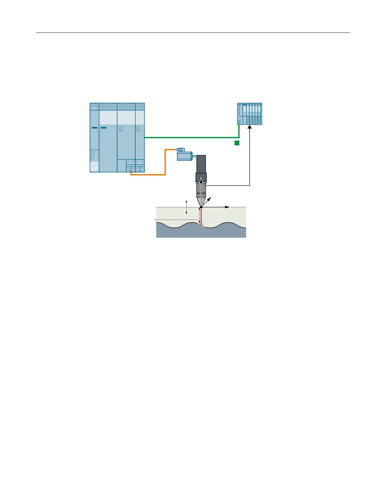
Clearance control (CLC/CLCX)

5.1 Brief description

System overview

The following figure provides an overview of the system components required for clearance

control:

1&8 ZLWK

6,0$7,& (7

6,2

6,1$0,&6 6

352),1(7 ,2

6HQVRU VLJQDO

/DVHU

0DFKLQLQJ KHDG ZLWK

FOHDUDQFH VHQVRU

0RWLRQ D[HV ; DQG <

&OHDUDQFH FRQWURO $[LV =

෥=

;

&OHDUDQFH WR EH

FRQWUROOHG

:RUNSLHFH VXUIDFH

Figure 5-1

System components for clearance control with SINUMERIK NCU

1D machining

For 1D machining, only one axis is influenced by the clearance control. For example, axis Z, as

shown in the machine configuration described in the system overview (see previous diagram).

Clearance control acts only in the direction of the Z axis.

3D machining

Three linear axes are used to position the tool. A detailed description can be found under 3D

clearance control - overview (Page 62).

Technologies

Function Manual, 10/2020, 6FC5397-8GP40-0BA1

Clearance control (CLC/CLCX)

5.2 Clearance control

5.2

Clearance control

5.2.1

POS mode

5.2.1.1

Overview

Properties of the POS mode

The system deviation of the clearance control is the difference between the programmed

setpoint clearance and the current actual clearance reported by the clearance sensor.

In POS mode this system deviation is calculated together with the actual position of the axis to

a target position for the clearance control axis. For this purpose, the delay time of the sensor in

relation to the actual position of the axis encoders must be compensated for in the best possible

way.

The POS mode does not cause overshooting, which depends on the size of the initial system

deviation, and is therefore more suitable for approaching from a greater distance than the GAIN

mode.

Technologies

Function Manual, 10/2020, 6FC5397-8GP40-0BA1

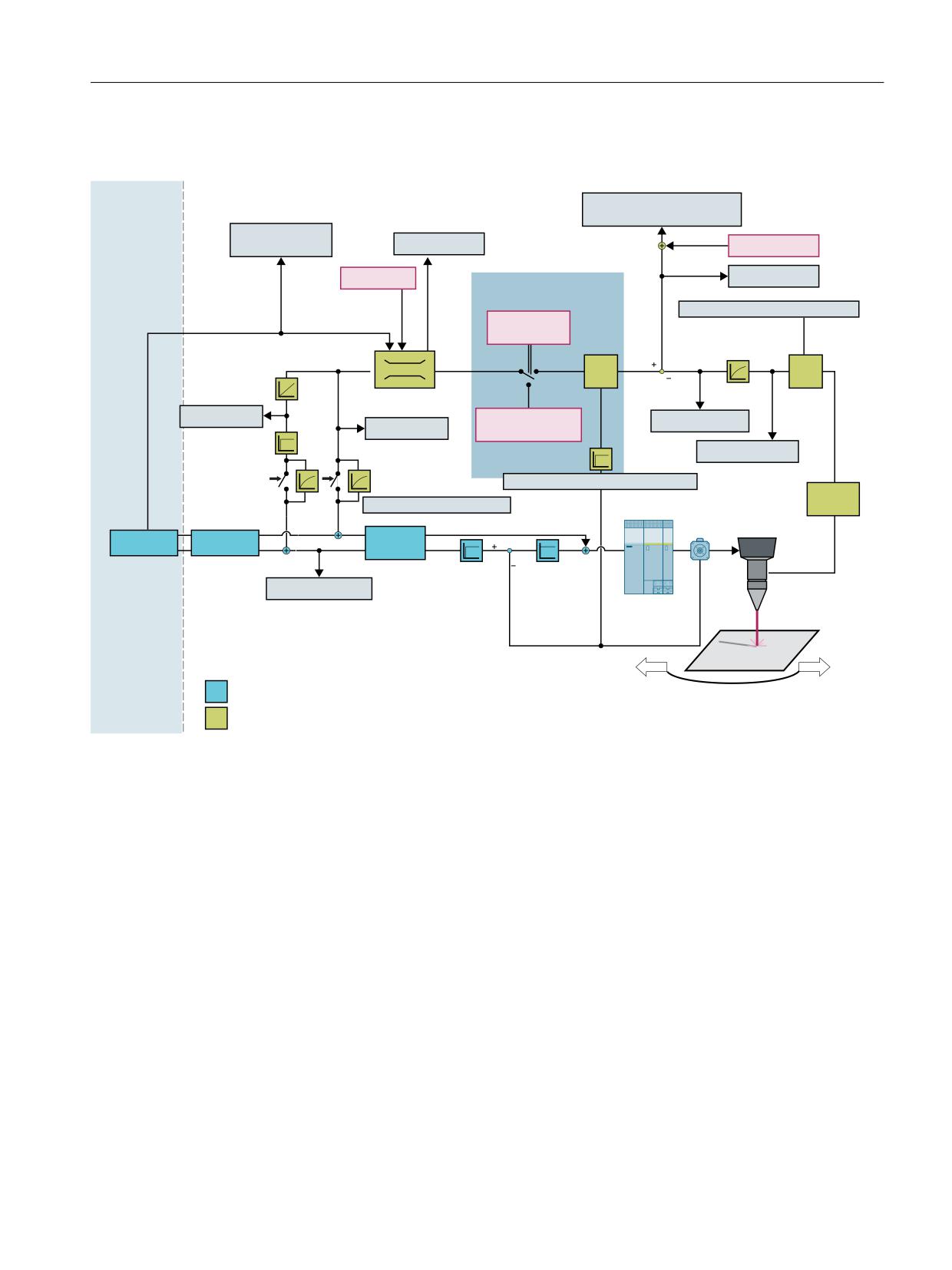
Clearance control (CLC/CLCX)

5.2 Clearance control

5.2.1.2

POS mode

,QWHUSRODWRU

3RVLWLRQ FRQWURO WDVN

%ORFN V\QF SURJ &/&B',67

WDVN

0&B&/&B',67$1&(B6(732,17

57'B833(5B/,0,7

57'B/2:(5B/,0,7

57'B'<1B/,0

57B',67B2))6(7

&/& 326 6<0

57B',5B/2&.

57'B352*B',67

$MC_CLC_SENSOR_FILTER_TIME[0]

57B7(&+B&0'

ಯMXPS SRVಯ

9ROWDJH GLVWDQFH

$[LV WUDYHO UDQJH DQG G\QDPLFV

UHPDLQLQJ IURP LQWHUSRODWHG PRWLRQ

WDEOHB

326

$YJ

PRGH

ILOWHU

/LPLWDWLRQ RI SRVLWLRQ

YHORFLW\ DQG DFFHOHUDWLRQ

57'B$&7B326

57B029(B326B5(/

57'B6(1625B',67

57'B$&7B9(/

57B029(B326B$%6

57'B6(1625B92/7

6ZLWFKHV ZLWK

3URIL1HW

$MC_CLC_SENSOR_DELAY_COMP_TIME

326 *$,1 PRGH

$MC_CLC_SENSOR_JERK_TIME

FRQYHUWHU

'ULYHV

DQDORJ

YHO

0RWRU

/DVHU KHDG

$;B-(5.

,32

),1( ,32

$;B'(/$<

SRV

&OHDUDQFH

)): 326

VHQVRU

6<0

57'B$&7B326B$%6

(QFRGHU

1&. 6\VWHP VRIWZDUH

,VRFKURQRXV

&/&; &RPSLOH &\FOH DGGRQ VRIWZDUH

Figure 5-2

POS mode

5.2.2

GAIN mode

5.2.2.1

Control dynamics - GAIN mode

Control loop gain K_V

The system deviation of the clearance control is the difference between the programmed

setpoint clearance and the current actual clearance reported by the clearance sensor. In GAIN

mode, this system deviation is multiplied by the control loop gain KV: The result is the control

speed that moves the axis toward the clearance setpoint.

The control loop gain KV_CLC in the superimposed sensor control loop is defined as:

Technologies

Function Manual, 10/2020, 6FC5397-8GP40-0BA1

Clearance control (CLC/CLCX)

5.2 Clearance control

6SHHG >PP PLQ@

.9_&/&

6\VWHP GHYLDWLRQ >PP@

Especially when approaching from a great distance, i.e. with an initially large system deviation,

the GAIN mode generates high control speeds which lead to overshooting of the axis position.

The maximum adjustable control loop gain is limited by the dynamics of the closed control loop

(sensor-control-axis) and the tolerable overshoot. Small values of the control loop gain cause

time losses due to a slow approach.

Max. control loop gain

The maximum achievable control loop gain is determined by the following delay and reaction

times of the overall system:

1. Reaction time of sensor

2. Delay time of the A/D converter

3. Delay/dead times of signal processing and transmission

4. Reaction time of position controller

5. Reaction times of speed and current controllers

6. Time constants of motor and mechanical system

Points 1, 3 and 4 are relevant in practice.

In total, the influencing variables result in an effective time constant. If the control loop gain is

set too high in relation to this time constant, natural oscillations of the axis/axes to be controlled

will occur in the range of a few hertz.

The aim of setting up the clearance control in GAIN mode is to adjust the decisive time constants

in such a way that the highest possible control loop gain can be set without the occurrence of

natural oscillations and with a tolerable overshoot amplitude when approaching.

Technologies

Function Manual, 10/2020, 6FC5397-8GP40-0BA1

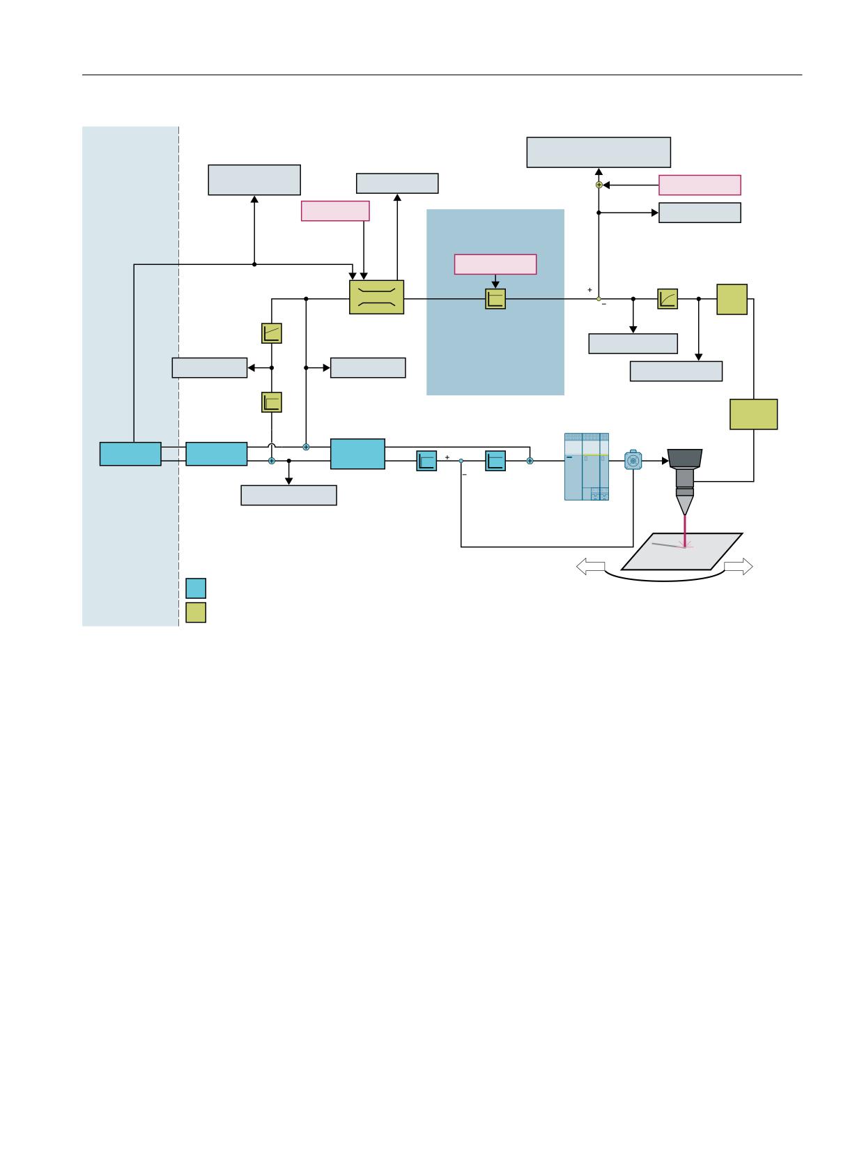
Clearance control (CLC/CLCX)

5.2 Clearance control

,QWHUSRODWRU WDVN

3RVLWLRQ FRQWURO WDVN

%ORFN V\QF SURJ &/&B',67

0&B&/&B',67$1&(B6(732,17

57'B833(5B/,0,7

57'B/2:(5B/,0,7

57'B'<1B/,0

57B',67B2))6(7

57B',5B/2&.

57'B352*B',67

57B*$,1B)$&725

$[LV WUDYHO UDQJH DQG G\QDPLFV

9ROWDJH GLVWDQFH

UHPDLQLQJ IURP LQWHUSRODWHG PRWLRQ

WDEOHB

$YJ

ILOWHU

/LPLWDWLRQ RI

0&B&/&B

SRVLWLRQ YHORFLW\

',67$1&(B&75/B*$,1

DQG DFFHOHUDWLRQ

57'B6(1625B',67

57'B$&7B326

57'B$&7B9(/

57'B6(1625B92/7

352),1(7

&/& 326 6<0

FRQYHUWHU

'ULYHV

DQDORJ

YHO

0RWRU

/DVHU KHDG

$;B-(5.

,32

),1( ,32

$;B'(/$<

SRV

&OHDUDQFH

)): 326

VHQVRU

6<0

57'B$&7B326B$%6

(QFRGHU

1&. 6\VWHP VRIWZDUH

,VRFKURQRXV

&/&; &RPSLOH &\FOH DGGRQ VRIWZDUH

Figure 5-3

GAIN mode

5.2.3

Dead times in the clearance control

Dead time

In order to achieve a highly dynamic control behavior, the clearance control is implemented in

the position controller cycle layer of the NC kernel.

For I/O modules that are connected via the isochronous fieldbus (PROFINET IRT) and when using

SINAMICS drives there is a system-dependent dead time T_deadof:

T_dead = 2 * position controller cycle + 2 * speed controller cycle + PROFINET T_i

In order to achieve an optimum dynamic response of the clearance control, the reaction time (or

dead time) of the sensor should not be significantly longer than the system-related dead time.

Technologies

Function Manual, 10/2020, 6FC5397-8GP40-0BA1

Clearance control (CLC/CLCX)

5.3 Technological features of clearance control

5.2.4

Optimizing the control behavior

If the control behavior of the axis becomes too hard due to feedforward control, the control

behavior can be optimized. Instructions for using the jerk filter can be found under Startup

(Page 38).

The speed filters of the SINAMICS S120 drive provide additional damping capabilities:

• Parameter 1414 ff. (time constant, speed setpoint filter 1, 2)

Note

Each damping measure in the axis control loop results in an additional contribution to the

increase of the total time constant of the superimposed sensor control loop!

Further information:

A complete description of the velocity feedforward control is provided in:

Function Manual Monitoring and compensating; Compensations, dynamic feedforward control

(following error compensation)

5.3

Technological features of clearance control

Clearance control is characterized by the following technological properties:

• Sensor characteristic

The voltage/clearance characteristic of a sensor can be specified with up to 16 breakpoints.

• Sensors

Several sensors with different gain characteristics can be used. The active sensor

characteristic can be switched over block-synchronously by means of a language command

in the part program.

• Control loop gain of the clearance control (GAIN mode)

The control loop gain of the clearance control, parameterized by NC machine data, can be

changed block-synchronously by a voice command in the part program. In addition, the real-

time variable CLC_RT_GAIN_FACTOR can multiply the gain.

• Motion limitation

The lower and upper limits configured in the NC machine data for the axis movements

induced by clearance control can be changed block-synchronously by means of a language

command in the part program.

An alarm appears when a limit is reached. The alarm response can be parameterized (stop of

the traversing motions or display only). The current position offset can be frozen via the real-

time variable CLC_RT_TECH_CMD (or a PLC signal).

• Switch-off behavior

The switch-off behavior of the clearance control can be programmed either with

synchronization to the current axis positions (no compensating motion) or with

compensating motion of the axes back to the last programmed IPO positions.

• Programmable clearance setpoint

The clearance setpoint can be programmed block-synchronously. An additional offset can be

added via the real-time variable CLC_RT_DIST_OFFSET.

Technologies

Function Manual, 10/2020, 6FC5397-8GP40-0BA1

Clearance control (CLC/CLCX)

5.4 Sensor collision monitoring

• State data of the clearance control

The following real-time variables can be read at any time:

CLC_RTD_SENSOR_VOLT, the current sensor signal in Volt

CLC_RTD_SENSOR_DIST, the distance calculated over the selected characteristic

• Sensor signal

The sensor signal can be smoothed by a sliding average value filter with adjustable time

constant:

62525 $MC_CLC_SENSOR_FILTER_TIME[0]

• Variables for synchronized actions

Additional functions such as jump-up or blocking of sensor motion can be controlled via the

real-time variable CLC_RT_TECH_CMD without having to switch the CLC function off and on

again.

5.4

Sensor collision monitoring

Tip-touch signal from the sensor

If the clearance sensor used has an additional "tip-touch" signal for detecting a collision of the

sensor with the workpiece to be machined, this signal can be made available to the clearance

control via a digital NC peripheral input.

As a reaction to this signal, the clearance control performs a fast retraction movement in all

clearance-controlled axes. The retraction movement is executed independently of the current

value of the velocity override at traversing velocity in positive control direction by a specified

distance. At the same time, the alert 75007 is issued and a real-time variable indicates the "tip-

touch" state. Synchronized actions can be used to program the desired reaction to the path. After

the cause of the collision has been eliminated, the retracted axis can be reset to control mode

via the real-time variable CLC_RT_TECH_CMD.

Parameterization

The digital peripheral input, which the tip-touch signal is wired to, is assigned to the clearance

control via the following machine data:

MD62504 $MC_CLC_SENSOR_TOUCHED_INPUT (digital peripheral input for "sensor collision"

signal)

The digital input is specified via the same input numbering that is used to address the

corresponding system variable $A_IN[input number].

If a negative input number is specified, the CLCX evaluates the tip-touch signal internally in

inverted form (wire break protection). In this case a falling signal edge triggers the tip-touch

reaction.

Internal tip-touch detection

If tip-touch detection is programmed, the clearance signal from the sensor can be monitored to

determine whether it falls below a set distance threshold: Machine data 62526

$MC_CLC_TIP_TOUCH_DISTANCE.

Technologies

Function Manual, 10/2020, 6FC5397-8GP40-0BA1

Clearance control (CLC/CLCX)

5.5 Startup

To avoid false tripping, the signal should be averaged over a suitable time (e.g. 30 ms) before

comparison with the distance threshold using the mean value filter available for this purpose:

Machine data 62525 $MC_CLC_SENSOR_FILTER_TIME[ 1 ].

The response of the CLCX to the undershooting of the tip-touch distance threshold is the same

as when an external tip-touch signal is received.

5.5

Startup

Compile cycle

Before setting up the technology function, ensure that the corresponding compile cycle has

been loaded and activated (see Installation and activation of loadable compile cycles (Page 17)).

General relationships

The clearance control works within the position controller task. The WCS and MCS positions on

the standard HMI screen do not show the offset generated by the clearance control. Only if you

switch off the CLC function with the CLC(0) command will the IPO positions displayed by default

be resynchronized, and thus the axis positions actually reached will be displayed.

The clearance control generates the overlaid movement within the CLC coordinate system:

• The zero point is the position at which the CLC function was activated.

• The arguments of CLC_LIM (<lower limit>, <upper limit>) refer to this coordinate system.

CLC_RTD_ACT_POS also refers to the CLC coordinate system.

Only the real-time variable CLC_RTD_ACT_POS_ABS shows the axis position in the regular

MCS coordinates. In the 3D case, this variable shows the same position as

CLC_RTD_ACT_POS.

Assign CLCX instance to a channel

A CLCX instance must be assigned to one channel each for activation. Several CLCX instances are

described under Multiple CLCX instances in one channel (Page 69).

Activating an instance in a channel

MD60940 $MN_CC_ACTIVE_IN_CHAN_CLCX[0] = 'H1'

• Bit n = 1

• n = channel number - 1

- Bit0 = 1st channel

- Bit1 = 2nd channel, etc.

Technologies

Function Manual, 10/2020, 6FC5397-8GP40-0BA1

Clearance control (CLC/CLCX)

5.5 Startup

Notes

If you want CLCX to act on a single axis only (and not in a 3D application), preferably do not

configure the CLC axis as a geometry axis ($MC_AXCONF_GEOAX_ASSIGN_TAB[2]=0).

This has the advantage that the position synchronization required when CLCX is deactivated

cannot affect XY path motion functions, but requires a change in programming.

When the Z axis is no longer a geometry axis, the geometry axis name of the Z axis (typically "Z")

can no longer be used to program rotating frames within the XY plane.

Therefore, program rotations with CRPL(1, 0) instead of CROT(Z, 0).

Jerk filter

Do not apply the standard jerk filter (MD32400 $MA_AX_JERK_ENABLE=0) to limit the axis jerk

caused by the CLCX motion, as this filter will cause a delay within the sensor control loop. If you

need to limit the axis jerk when moving the axis with the regular interpolator, program SOFT

movement mode instead and limit the jerk with MD32431 $MA_MAX_AX_JERK.

CLCX provides a separate jerk filter (MD62518 $MC_CLC_SENSOR_JERK_TIME) to limit the jerk

during CLCX jerk movements. If a filter time constant greater than zero is set there, the CLCX

automatically switches the filter on and off in a sliding manner according to the current situation:

• The jerk filter is switched on when approaching the plate and in case of predefined "jumps"

of the axis; in normal sensor-controlled control operation it is switched off. Nevertheless, the

specified filter time should also be kept as short as possible for this jerk filter (in the <20 ms

range).

5.5.1

Setup steps

Setting up CLCX

To set up CLCX for optimum performance and productivity, it is recommended that the following

steps be performed:

• Optimize the axis/axes by setting up Feed-Forward, DSC and other functions that provide the

best possible precision and dynamics.

• Set up the analog input of the sensor for isochronous operation (PROFINET IRT), see Setting

up the analog sensor input (Page 41).

Technologies

Function Manual, 10/2020, 6FC5397-8GP40-0BA1

Clearance control (CLC/CLCX)

5.5 Startup

• Linearize the clearance sensor input using the machine data tables

62510__MC_CLC_SENSOR_VOLTAGE_TABLE_1[0... 15] and

62511__MC_CLC_SENSOR_DIST_TABLE_1[0...15], see also Linearizing the signal of the

clearance sensor (Page 44).

- To obtain optimum performance of the CLCX function, the sensitive clearance range of

the sensor should be as large as possible (preferably up to 20 mm) and linearized as well

as possible.

- The highest entry in the clearance table and the correct linearization of the distance

within the entire table range are particularly important in order to obtain the optimum

sensor-controlled approach movement from a far-away starting position to the workpiece

surface.

- The linearization of the sensor characteristic curve can be automated with an appropriate

part program. CLCX simplifies a quick sensor calibration check, since both the analog

input voltage information and the resulting clearance of the currently selected table

available are available, even when CLCX is switched off.

• When using the POS mode and the enhanced approach function, the following is

recommended:

- The time delay between the relative position measurement of the sensor and the absolute

axis position detection of the encoder must be compensated for in the best possible way,

see Compensation of the time delay of the sensor (Page 45).

• The commissioning and testing of all functions that do not directly depend on the axis

dynamics and the specific sensor characteristic can also be carried out via Create MyVirtual

Machine with simulated axes and a simulated sensor.

5.5.2

Activating the technological function

The technology function is activated via the machine data:

MD60940 $MN_CC_ACTIVE_IN_CHAN_CLCX[0], bit n = 1

n = channel number - 1; Bit0 = 1st channel, Bit1 = 2nd channel, etc.

Note

A maximum of four instances of the CLCX technology function can be activated on one NCU.

Technologies

Function Manual, 10/2020, 6FC5397-8GP40-0BA1

Clearance control (CLC/CLCX)

5.5 Startup

5.5.3

Configuring the memory

The CLCX technology function requires additional data in the NC-internal block memory. For

each CLCX instance that is active in the channel, the values specified must be entered in the

following memory-configuring channel-specific machine data. If the memory requirement for

other compile cycle functions is already entered in this MC, the values must be added to the

existing entries:

• MD28090 $MC_MM_NUM_CC_BLOCK_ELEMENTS: + 4(number of block elements for

compile cycles)

• MD28100 $MC_MM_NUM_CC_BLOCK_USER_MEM: + 20(size of block memory for compile

cycles (DRAM), in KB)

5.5.4

Sensor input and sensor signals

5.5.4.1

Setting up the analog sensor input

Recommended hardware

It is recommended to convert and read in the analog input signals of the capacitive clearance

sensor with the following hardware:

Table 5-1

Recommended SIMATIC modules

Article number

Device

Description

6ES7 151-3BA60-0AB0

SIMATIC ET200S IM151-3PN HS Firmware

Profinet Interface Module

V3.0

6ES7 138-4CA01-0AA0

SIMATIC ET200S PM-E DC24V

Power Module

6ES7 134-4FB52-0AB0

SIMATIC ET200S 2AI U HS

Module with 2 analog inputs

In order to achieve the best dynamic response of the clearance control, the analog input, which

contains the clearance information, must be isochronously transferred to the NC.

Configure the PROFINET IRT operation in the "HWConfig" area of the Simatic Manager or in the

corresponding function of the TIA Portal for:

• the bus segment

• the interface module (the head module)

• the analog input module to which the sensor is connected

• the digital input for tip-touch detection of the sensor - if available

Technologies

Function Manual, 10/2020, 6FC5397-8GP40-0BA1

Clearance control (CLC/CLCX)

5.5 Startup

5.5.4.2

Parameterizing the input signals

The following input signals must be parameterized in the machine data:

• Input voltage of the clearance sensor

1 analog input

• "Sensor-tip-touch" input signal (optional)

1 digital input

Analog input

The PROFINET address of the analog input module configured on the PLC side must be entered

on the NC side in the following machine data:

• MD10362 $MN_HW_ASSIGN_ANA_FASTIN (per analog input) (hardware assignment of the

fast analog NC inputs)

Digital input

Unless one of the onboard inputs of the NCU is used for this purpose, the PROFINET address of

the digital input module configured on the PLC side must be entered in the following machine

data:

• MD10366 $MN_HW_ASSIGN_DIG_FASTIN (per -bit input block) (hardware assignment of the

external digital NC inputs)

A complete description of the analog and digital inputs can be found in:

Further information

Function Manual Basic Functions; digital and analog NC I/O

5.5.4.3

Simulation of the sensor signals

Preparing a simulation

The properties of the single-axis CLCX can be tested without a real clearance sensor and, if

necessary, even without real axes. In this case, a sensor/plate simulation integrated in the CLCX

software closes the control loop.

The axes are switched to simulation mode as usual with the following machine data:

•

30240__$MA_ENC_TYPE[Z]=0

•

30130__$MA_CTRLOUT_TYPE[Z] =0

The simulation can only simulate the fundamental function of the sensor, but not the real

dynamic response of the clearance control.

To apply the simulation, the following definitions must be added to the definition file, which also

contains the other GUD definitions of the CLCX:

• DEF CHAN REAL CLC_SIM_SHEET_POS[3]

• DEF CHAN REAL CLC_SIM_SENSOR_DELAY[2]

Technologies

Function Manual, 10/2020, 6FC5397-8GP40-0BA1

Clearance control (CLC/CLCX)

5.5 Startup

A restart of the NC kernel is required for the new GUD definitions to take effect in the CLCX. Then

the simulation of sensor and sheet metal (workpiece) can be used.

Defining the sensor simulation

The simulation only works if a simulated sensor delay time not equal to zero is set in the

following GUD variable:

Programming example

CLC_SIM_SENSOR_DELAY[0] = 0.001234

; activates the simulation and uses a simulated

; sensor delay of 1.234 ms

Note

The content of the GUD variable CLC_SIM_SENSOR_DELAY[0] is intentionally deleted after each

NC restart to deactivate the sensor simulation by default after the restart. This is to avoid the

accidental use of the simulated sensor when a real sensor is connected.

Defining the sheet metal

To simulate the sheet metal, simply enter the desired sheet metal position in MCS coordinates

into this GUD variable:

Programming example

CLC_SIM_SHEET_POS[0] = -30 ; simulates a sheet metal in the MCS position -30 mm.

Make sure that the simulated sheet metal is positioned UNDER the axis position where you

switch on the CLC.

The other GUD elements can be applied optionally:

Programming example

CLC_SIM_SHEET_POS[2] = 0.005

;simulates white noise of the sheet metal position of 5 µm

CLC_SIM_SHEET_POS[1] = 0.1

; simulates a linear up/down movement of the sheet metal of

0.1 mm.

CLC_SIM_SENSOR_DELAY[1] = 2.0

; .. with a duration of 2 seconds

If you change the content of a GUD variable within a part program, note that it may take a short

time until the CLCX actually evaluates a changed GUD value.

In order to obtain stable test conditions, it is therefore recommended to program a dwell time

of one second (G4 F1) after a change of the GUD values or before switching on or enabling the

CLCX motion.

In order for the simulation of the closed CLC control loop to behave as realistically as possible

dynamically, you should compensate the set delay of the simulated sensor in the machine data

$MC_CLC_SENSOR_DELAY_COMP_TIME in the same way as is required for a real sensor:

$MC_CLC_SENSOR_DELAY_COMP_TIME = CLC_SIM_SENSOR_DELAY[0]

Technologies

Function Manual, 10/2020, 6FC5397-8GP40-0BA1

Clearance control (CLC/CLCX)

5.5 Startup

5.5.4.4

Linearizing the signal of the clearance sensor

Normalizing the analog input value

The first step in providing a linearized sensor signal is to normalize the analog input value:

• Connect a known static analog voltage to the sensor input.

• Adjust the value of MD62503 $MC_CLC_ANALOG_IN_HW_NORM_FACT until the variable

CLC_RTD_SENSOR_VOLT correctly indicates the voltage in V applied at the input.

This can also be done without the CLCX being switched on by program command, as the

variable is updated as soon as CLCX is activated via the PowerOn machine data.

• The same applies to the variable CLC_RTD_SENSOR_DIST, which displays the linearized

sensor distance resulting from the applied input voltage with the currently effective sensor

characteristic curve:

MD62510 $MC_CLC_SENSOR_VOLTAGE_TABLE_1[0... 15] MD62511

$MC_CLC_SENSOR_DIST_TABLE_1[0... 15]

MD62512 $MC_CLC_SENSOR_VOLTAGE_TABLE_2[0... 15] MD62513

$MC_CLC_SENSOR_DIST_TABLE_2[0... 15]

Calibration of the sensor table via "CLC_RTD_SENSOR_VOLT" and "CLC_RTD_SENSOR_DIST"

Recalibrating the sensor means storing the currently effective characteristic of the sensor in a

CLCX sensor characteristic curve. For this purpose, the distance breakpoints to be measured are

first selected by entering them in ascending order starting with zero, e.g. in the table values of

the machine data $MC_CLC_SENSOR_DISTANCE_TABLE_1. In areas where the characteristic

curve is strongly non-linear, a correspondingly higher number of breakpoints should be selected.

Starting with the zero distance, at which the sensor should almost touch the sheet metal, the

axis is moved upwards step by step by the entered distances via a part program with the CLCX

function switched off. For each distance the voltage output by the sensor is written to the

corresponding element of the voltage table $MC_CLC_SENSOR_VOLTAGE_TABLE_1.

• Start with the greatest possible approximation

Greatest possible approximation means almost contact of the sensor with the sheet metal

(zero distance).

• Gradually increase the distance and transfer the measured voltage to the element of the

voltage table corresponding to the distance.

Note

• The first entry within the clearance table must be zero. If it is not possible to measure the

sensor voltage at this (contact) position, a corresponding estimated sensor voltage should be

entered in MD62510 $MC_CLC_SENSOR_VOLTAGE_TABLE_x[0].

• All subsequent clearance and voltage entries must be monotonically increasing.

The table ends with the entry in index 15 or with a clearance entry of 0.0 under an index smaller

than 15.

Technologies

Function Manual, 10/2020, 6FC5397-8GP40-0BA1

SINUMERIK 840D sl. Service - Functions. Manual (2018-2020) - page 77