SINUMERIK 840D sl. Service - Functions. Manual (2018-2020) - page 35
K3: Compensations
5.5 Interpolatory compensation
The compensation values and additional table parameters are entered in the compensation
tables using special system variables. Data can be loaded in two different ways:
● By starting an NC program with the parameter values.
● By transferring the compensation tables from an external computer to the control.
Note
The respective compensation tables can only be loaded if the corresponding compensation
function is not active for all axes:
● MD32700 $MA_ENC_COMP_ENABLE[<axis>] == 0
● MD32710 $MA_CEC_ENABLE[<axis>] == 0
As the compensation data is also retained when the controls are switched off.
Note
When changing machine data:
● MD18342 $MN_MM_CEC_MAX_POINTS
● MD38000 $MA_MM_ENC_COMP_MAX_POINTS
is formatted during the next system run-up of the static user memory (see Section "S7: Memory
configuration (Page 827)").
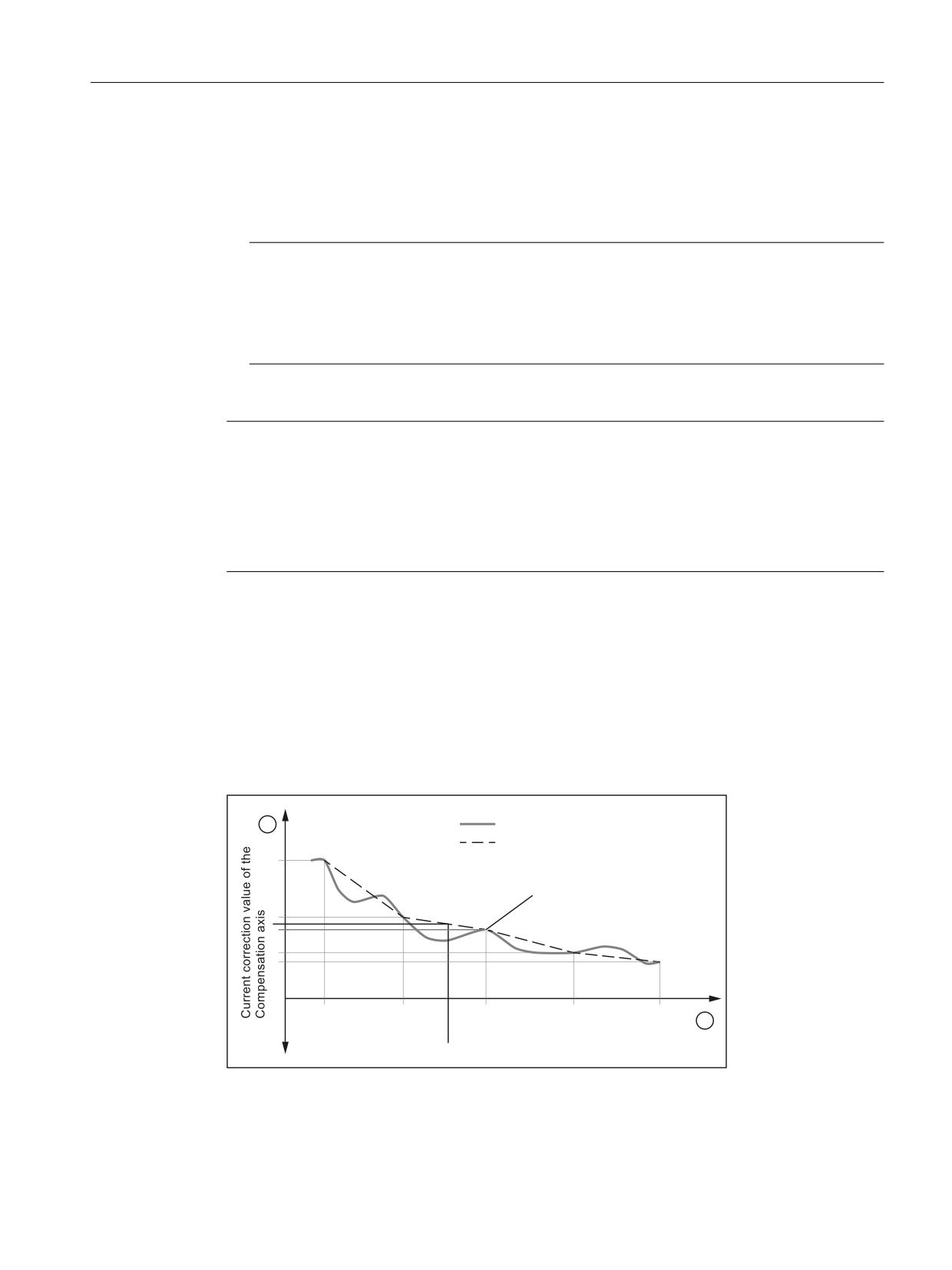
Interim value calculation
The traversing distance defined via the start and end position within which compensation is to
apply, is divided into several sub-paths of equal size. The number of sub-paths is defined
depending on the error curve and the desired precision. The positions that limit these sub-
paths are referred to as interpolation points below. An interpolation and a compensation value
must be assigned to each interpolation point. Between two interpolation points, the effective
compensation value is determined by linear interpolation.
(UURU FXUYH
&RPSHQVDWLRQ FXUYH
,QWHUSRODWLRQ SRLQW
Q
Q
Q
Q
Q
&XUUHQW SRVLWLRQ RI EDVLF D[LV
① Compensation values of the compensation axis
② Position of basic axis
Figure 5-12
Intermediate value calculation by linear interpolation
Extended Functions
Function Manual, 12/2018, A5E40874029B AB
279
K3: Compensations
5.5 Interpolatory compensation
Supplementary conditions
Compensation value at reference point
It is recommended that a compensation table be structured in such a way that the
compensation value has the value "0" at the reference point of the axis.
5.5.2
Leadscrew error and measuring system error compensation
5.5.2.1
Measuring system error compensation (MSEC)
Leadscrew and measuring system errors
The measuring principle of "indirect measurement" on NC-controlled machines is based on
the assumption that the lead of the ball screw is constant at any point within the traversing
range, so that the actual position of the axis can be derived from the position of the drive spindle
(ideal case). However, manufacturing tolerances result in dimensional deviations of varying
degrees of severity on spindles (so-called leadscrew errors).
Added to this are the dimensional deviations (differences in reference division) caused by the
measuring system as well as its mounting on the machine (so-called measuring system errors),
plus any machine-dependent error sources.
Compensation
With "measuring system error compensation" (referred to below as MSEC), the base and
compensation axes are always identical. It is therefore an axial compensation for which a
definition of the base axis and compensation axis in the compensation table is not necessary.
Note
The leadscrew error compensation (LEC) is part of the measuring system error compensation.
The principle of the MSEC is to modify the axis-specific position actual value by the assigned
compensation value in the interpolator clock cycle and to apply this value to the machine axis
for immediate traversal. A positive compensation value causes the corresponding machine
axis to move in the negative direction.
The magnitude of the compensation value is not limited and is not monitored. In order to avoid
impermissibly high velocities and accelerations caused by compensation, small compensation
values must be selected. Large compensation values can cause other axis monitoring
functions to output alarms (e.g. contour monitoring, speed setpoint limitation).
If the axis to be compensated has a 2nd position measuring system, a separate compensation
table must be created and activated for each measuring system. The correct table is
automatically used when switching between measuring systems.
Extended Functions
280
Function Manual, 12/2018, A5E40874029B AB
K3: Compensations
5.5 Interpolatory compensation
Preconditions / activation
The MSEC is only active until the following pre-conditions:
● The compensation values are stored in the static user memory and are active (after POWER
ON).
● The function has been activated for the relevant machine axis:
MD32700 $MA_ENC_COMP_ENABLE [<e>] = 1
with: <e>
= Position measuring system
<e> = 0
Measuring system 1
<e> = 1
Measuring system 2
● The axis has been referenced:
DB31, ... DBX60.4 or 60.5 =1 (referenced/synchronized 1 or 2)
As soon as these conditions have been fulfilled, the axis-specific actual value is modified by
the compensation value in all modes and traversed by the machine axis immediately.
If the reference is then lost, e.g. because the encoder frequency has been exceeded (DB31, ...
DBX60.4 or 60.5 = 0), compensation processing is deactivated.
5.5.2.2
Commissioning
Machine data
Number of compensation interpolation points
Chinese axis - The number of compensation table interpolation points must be stated for each
measuring system:
MD38000 $MA_MM_ENC_COMP_MAX_POINTS[<e>,<AXi>]
● <e>: Position measuring system
● <AXi>: axis
The number of interpolation points of a compensation table is calculated from the
accompanying system variables (see below):
● End position: $AA_ENC_COMP_MAX[...]
● Start position: $AA_ENC_COMP_MIN[...]
● Distance between interpolation points: $AA_ENC_COMP_STEP[...]
Number of interpolation points = ((end position - start position) / interpolation point distance)
+ 1
Extended Functions
Function Manual, 12/2018, A5E40874029B AB
281
K3: Compensations
5.5 Interpolatory compensation
System variables
For each machine axis as well as for each measuring system (if a 2nd measuring system
exists), the position-related compensation values as well as additional table parameters should
be saved for every compensation relationship in the form of system variables:
● $AA_ENC_COMP_MIN[<e>,<AXi>] (initial position)
The initial position is the axis position at which the compensation table for the relevant axis
begins (≙ interpolation point 0).
The compensation value for the initial position is $AA_ENC_COMP[<e>,0,<AXi>)].
The compensation value of interpolation point 0 is used for all positions smaller than the
initial position (does not apply for tables with modulo function).
● $AA_ENC_COMP_MAX[<e>,<AXi>] (end position)
The end position is the axis position at which the compensation table for the relevant axis
ends (≙ interpolation point <k>).
The compensation value for the end position is $AA_ENC_COMP[<e>,<k>,<AXi>)].
The compensation value of interpolation point is used for all positions larger than the end
position (exception for table with modulo function).
The following supplementary conditions apply to interpolation point <k>:
- for k = MD38000 - 1:
The compensation table is fully utilized!
- for k < MD38000 - 1:
The compensation table is not fully utilized. Compensation values entered in the table
that are greater than k are ignored.
- for k > MD38000 - 1:
The compensation table is limited by a control function which reduces the end position.
Compensation values that are greater than k are ignored.
● $AA_ENC_COMP_STEP[<e>,<AXi>] (distance between interpolation points)
The distance between interpolation points defines the distance between the compensation
values in the relevant compensation table.
Extended Functions
282
Function Manual, 12/2018, A5E40874029B AB

K3: Compensations
5.5 Interpolatory compensation
●
$AA_ENC_COMP[<e>,<N>,<AXi>] (correction value for interpolation point N of the
compensation table)
<N> = interpolation point (axis position)
For every individual interpolation point the compensation value must be entered in the table.
<N> is limited by the maximum number of interpolation points of the particular compensation
table (MD38000 $MA_MM_ENC_COMP_MAX_POINTS):
0 ≤ N ≤ MD38000 -1
The size of the compensation value is not limited.
Note
The first and last compensation values remain active over the entire traversing range;
i.e. these values should be set to "0" if the compensation table does not cover the entire
traversing range.
●
$AA_ENC_COMP_IS_MODULO[<e>,<AXi>] (compensation with modulo function)
System variable to activate/deactivate the compensation with modulo function:
- $AA_ENC_COMP_IS_MODULO[<e>,<AXi>] = 0: Compensation without modulo
function
- $AA_ENC_COMP_IS_MODULO[<e>,<AXi>] = 1: Compensation with modulo function
When compensation with modulo function is activated, the compensation table is repeated
cyclically, i.e. the compensation value at position $AA_ENC_COMP_MAX (≙ interpolation
point $AA_ENC_COMP[<e>,<k>,<AXi>]) is immediately followed by the compensation
value at position $AA_ENC_COMP_MIN (≙ interpolation point
$AA_ENC_COMP[<e>,<0>,<AXi>]).
For rotary axes with modulo 360° degrees it is therefore suitable to program 0°
($AA_ENC_COMP_MIN) as the initial position and 360° ($AA_ENC_COMP_MAX) as the
end position.
The compensation values entered for these two positions should be the same as otherwise
the compensation value jumps from MAX to MIN at the transition point and vice versa.
CAUTION
Wrong correction values
When writing the correction values for a correction table, it must be ensured that all
interpolation points within the parameterized range are assigned a value. Correction
values which are not described otherwise contain random values.
Extended Functions
Function Manual, 12/2018, A5E40874029B AB
283
K3: Compensations
5.5 Interpolatory compensation
Note
Table parameters containing position information are automatically converted when the
system of units is changed (change from MD10240
$MN_SCALING_SYSTEM_IS_METRIC).
The position information is always interpreted in the current measuring system. Conversion
must be implemented externally.
Automatic conversion of the position data can be configured as follows:
MD10260 $MN_CONVERT_SCALING_SYSTEM = 1
External conversion is no longer necessary.
References:
Function Manual Basic Functions; Velocities, Setpoint/Actual Value Systems, Closed-Loop
Control (G2)
5.5.2.3
Example
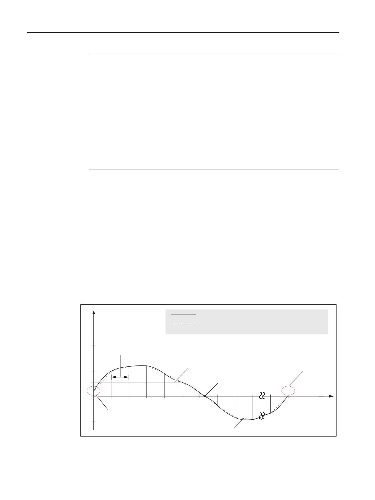
Sample parameterization of a compensation table:
● Machine axis: X1
● Measuring system: 1
● Starting position: -200 mm
● End position: 600 mm
● Distance between interpolation points: 1 mm
● Number of interpolation points: MD38000 $MA_MM_ENC_COMP_MAX_POINTS = ((600
- -200) / 1) + 1 = 801
The memory requirement in the static user memory is: 801 * 8 Byte = 6408 Byte
(UURU FXUYH
2IIVHW YDOXH
&RPSHQVDWLRQ FXUYH
OLQHDU LQWHUSRODWLRQ EHWZHHQ LQWHUSRODWLRQ SRLQWV
,QWHUSRODWLRQ SRLQW GLVWDQFH
1XPEHU RI LQWHUSRODWLRQ SRLQWV
$$B(1&B&203
0'
0$B00B(1&B&203B0$;B32,176 ุ
2IIVHW YDOXH DW
(QG SRVLWLRQ
LQWHUSRODWLRQ SRLQW
$$B(1&B&203B0$;
2IIVHW YDOXH DW
UHIHUHQFH SRLQW
$[LV SRVLWLRQ
,QWHUSRODWLRQ
SRLQW
6WDUWLQJ SRVLWLRQ
$$B(1&B&203B0,1
OLQHDU LQWHUSRODWHG LQWHUPHGLDWH YDOXHV
Extended Functions
284
Function Manual, 12/2018, A5E40874029B AB
K3: Compensations
5.5 Interpolatory compensation
Program for writing system variables
Program code
Comment
%_N_AX_EEC_INI
CHANDATA(1)
$AA_ENC_COMP[0,0,X1]=0.003
1st compensation value (interpolation point 0):
+3μm
$AA_ENC_COMP[0,1,X1]=0.01
2nd compensation value (interpolation point 1):
+10μm
$AA_ENC_COMP[0,2,X1]=0.012
3rd compensation value (interpolation point 2):
+12μm
$AA_ENC_COMP[0,800,X1]=-0.0
Last compensation value (interpolation point
800): 0μm
$AA_ENC_COMP_STEP[0,X1]=1.0
Distance between interpolation points 1.0 mm
$AA_ENC_COMP_MIN[0,X1]=-200.0
Compensation starts at -200.0 mm
$AA_ENC_COMP_MAX[0,X1]=600.0
Compensation ends at +600.0 mm
$AA_ENC_COMP_IS_MODULO[0,X1]=0
Compensation without modulo function
M17
5.5.3
Sag and angularity error compensation
5.5.3.1
General information
Function
The sag and angularity error compensation (cross error compensation, CEC) is an axis-specific
compensation, where a correction and/or compensation value is added to the the setpoint
position of the compensation axis. The compensation value is derived from the current setpoint
position of one or several basic axes.
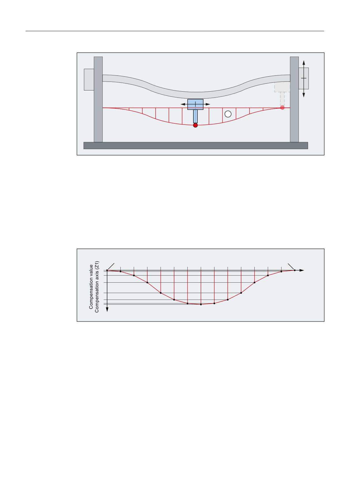
● Sag errors
In the case of sag errors, the weight of a machine part or workpiece leads to a position-
dependent error in the tool center point (TCP).
● Angularity errors
For angularity errors, a deviation in the ideal angle in the geometric axes in relation to each
other leads to a position-dependent error in the tool center point (TCP).
Extended Functions
Function Manual, 12/2018, A5E40874029B AB
285
K3: Compensations
5.5 Interpolatory compensation
=
<
7&3
① Position error in Z1 as a function of the position of Y1
Figure 5-13
Example: Sag errors
Error compensation
For error compensation, at various interpolation points (setpoint positions) of the basic axis
(Y1), the particular position error should be determined and entered into the compensation
table. When the basic axis (Y1) traverses, in the interpolation clock cycle, the control system
calculates the actual compensation value for the compensation axis (Z1) by linearly
interpolating between the points. The compensation value is added to the setpoint of the
compensation axis (Z1). A positive compensation value causes the compensation axis (Z1) to
traverse in the negative direction.
6HWSRLQW SRVLWLRQ EDVLF D[LV <
6WDUWLQJ SRVLWLRQ
(QG SRVLWLRQ
,QWHUSRODWLRQ SRLQWV
Figure 5-14
Compensation table
Summed compensation value
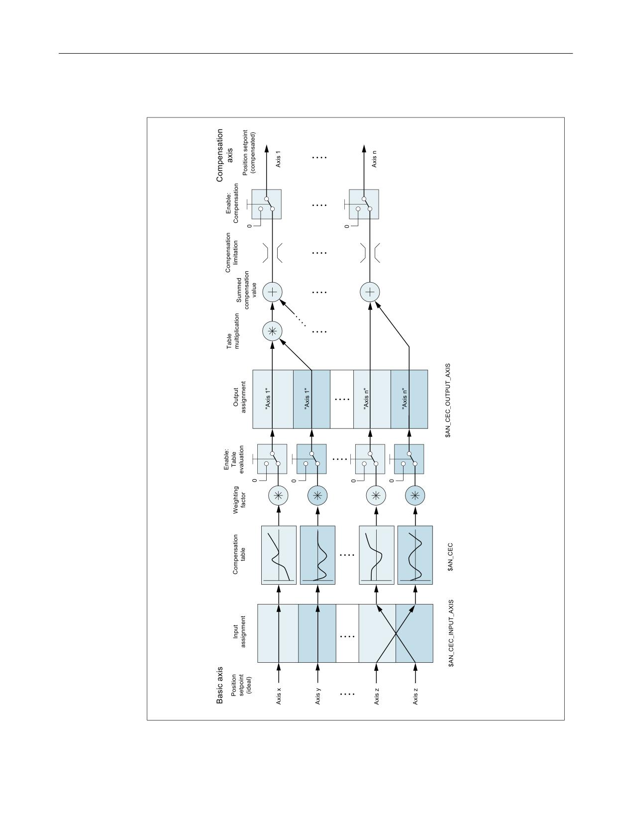
Compensation values from several compensation tables can be applied to a compensation
axis. The resulting summed compensation value is the sum of all of the individual
compensation values.
Parameterization options
● Anaxis can be defined as a basic axis for severalcompensation tables.
● Severalcompensation tables can act on onecompensation axis. The total (summed)
compensation value is derived from the sum of the compensation values of the individual
compensation tables.
Extended Functions
286
Function Manual, 12/2018, A5E40874029B AB

K3: Compensations
5.5 Interpolatory compensation
● An axis can be both a base axis and a compensation axis at any one time. The programmed
position setpoint is used to calculate the compensation values.
● The scope of action of the compensation (starting and end position of the base axis) and
the distance between the interpolation points can be defined for every compensation table.
● The compensation can act as a function of the direction.
● Every compensation table has a modulo function for cyclic evaluation.
● A weighting factor can be taken into account for each compensation table, with which the
value in the table is multiplied.
● Using table multiplication, the actual compensation value KA of compensation table A can
be multiplied with the actual compensation value Kx of any arbitrary compensation table X,
i.e. also with itself. The result of the table multiplication is added to the actual compensation
value KA of compensation table A, and this is then the sum compensation value SKA, which
is then effective in the compensation axis.
SKA = KA + KA * Kx
● Axes-specific activation for all compensation relationships of the axis via the machine data:
MD32710 $MA_CEC_ENABLE[<axis>]
● Table-specificactivation via the setting data:
SD41300 $SN_CEC_TABLE_ENABLE[<table>]
Application example: Processing-dependent change to the compensation ratio by switching
the active compensation table via part program/synchronous actions or PLC user program.
Application examples
Compensation of repetitive errors with short wavelength
To compensate for repetitive errors with short wavelength in an axis, a compensation table
with modulo function for the repetitive error components (short wavelength) together with a
second compensation table without modulo function for the aperiodic error component are
parameterized for the same axis.
User-specific leadscrew error compensation
For user-specific leadscrew error compensation, a compensation table with the same axis is
parameterized as basic and compensation axis.
However, in this case there is a disadvantage in so much that contrary to the standard function
a measuring system switchover cannot be automatically taken into consideration.
5.5.3.2
Commissioning: Machine data
Number
Identifier
Meaning
NC-specific machine data
MD10240
$MN_SCALING_SYS-
Metric basic system
TEM_IS_METRIC.
MD10260
$MN_CONVERT_SCAL-
Basic system switchover active
ING_SYSTEM
Extended Functions
Function Manual, 12/2018, A5E40874029B AB
287

K3: Compensations
5.5 Interpolatory compensation
Number
Identifier
Meaning
MD18342
$MN_MM_CEC_MAX_POINTS
Number of interpolation points per compensation ta-
ble
Axis-specific machine data
MD32710
$MA_CEC_ENABLE
Enabling sag compensation
MD32711
$MA_CEC_SCALING_SYS-
System of units for sag compensation
TEM_METRIC
MD32720
$MA_CEC_MAX_SUM
Maximum compensation value for sag compensation
MD32730
$MA_CEC_MAX_VELO
Maximum velocity change for CEC
System of units (MD10240, MD10260, MD32711)
The system of units effective in the control system (metric or inch) is defined using:
MD10240 $MN_SCALING_SYSTEM_IS_METRIC = <system of units>
System of units switchover without automatic conversion
Table parameters with position data are automatically converted if the system of units changes.
The position data is always interpreted in the actual system of units. Conversion must be
implemented externally.
System of units switchover with automatic conversion
The automatic conversion of position data is activated using:
MD10260 $MN_CONVERT_SCALING_SYSTEM = TRUE
As a consequence, the system of units set in the following machine data is effective for all
compensation tables of the axis:
MD32711 $MA_CEC_SCALING_SYSTEM_METRIC = <system of units>
As a consequence, all position data is interpreted together with the summed compensation
value in the configured system of units. External conversion of position data is no longer
necessary when the system of units changes.
Axes-specific activation (MD32710)
Axis-specific activation for all compensation relationships of the axis is realized using:
MD32710 $MA_CEC_ENABLE[<axis>] = TRUE
Number of interpolation points per compensation table (MD18342)
The number of interpolation points per compensation table is parameterized using:
MD18342 $MN_MM_CEC_MAX_POINTS[<table index>] = <number of interpolation points>
The number of interpolation points required in a compensation table is calculated from the
maximum, minimum and step width (increment) set in System variables (Page 290) of table:
<Number of interpolation points> = ($AN_CEC_MAX - $AN_CEC_MIN) / $AN_CEC_STEP +
1
Extended Functions
288
Function Manual, 12/2018, A5E40874029B AB

K3: Compensations
5.5 Interpolatory compensation
Monitoring (MD32720, MD32730)
Absolute limiting
To avoid inadmissibly high compensation motion of the compensation axis, the summed
compensation value is monitored against the maximum value specified in the machine data:
MD32720 $MA_CEC_MAX_SUM[<compensation axis>] = <maximum value>
When the value is exceeded, the summed compensation value is limited to the maximum value
and alarm 20124 "Summed compensation value too high" is displayed.
Limiting the change
To avoid inadmissibly high dynamic loads on the compensation axis, the summed
compensation value change is monitored against the maximum value specified in machine
data:
MD32730 $MA_CEC_MAX_VELO[<compensation axis>] = <percentage of the maximum axis
velocity (MD32000 $MA_MAX_AX_VELO)>
When exceeded, the summed compensation value change is limited to the maximum value
and alarm 20125 "Compensation value change too fast" is displayed.
The reduced traversing distance as result of the limiting is output as soon as the compensation
value is no longer being limited.
5.5.3.3
Commissioning: Setting data
Number
Identifier
Meaning
SD41300
$SN_CEC_TABLE_ENABLE
Compensation table enable
SD41310
$SN_CEC_TABLE_WEIGHT
Weighting factor
Compensation table enable (SD41300)
The evaluation of the compensation table is enabled using the setting data:
SD41300 $SN_CEC_TABLE_ENABLE[<table index>] = TRUE
The compensation value determined using the compensation table is only added to the
summed compensation value of the compensation axis when the evaluation is enabled.
Weighting factor (SD41310)
The weighting factor should be entered in the setting data, with which the compensation value
determined from the compensation table is multiplied:
SD41310 $SN_CEC_TABLE_WEIGHT[<table index>] = <weighting factor>
As standard, the weighting factor has a value of 1.0. The compensation table becomes inactive
with a weighting factor of 0.0.
Extended Functions
Function Manual, 12/2018, A5E40874029B AB
289

K3: Compensations
5.5 Interpolatory compensation
5.5.3.4
Commissioning: System variable
Identifier
Meaning
NC-specific system variables
$AN_CEC
Compensation values
$AN_CEC_DIRECTION
Direction dependency
$AN_CEC_INPUT_AXIS
Basic axis
$AN_CEC_INPUT_NCU
Basic axis on the NCU:
$AN_CEC_IS_MODULO
Modulo function
$AN_CEC_MAX
End position
$AN_CEC_MIN
Starting position
$AN_CEC_MULT_BY_TABLE
Multiplication
$AN_CEC_OUTPUT_AXIS
Compensation axis
$AN_CEC_OUTPUT_NCU
Compensation axis on the NCU
$AN_CEC_STEP
Distance between interpolation points
$AN_CEC_TYPE
Table type
Axis-specific system variables
$VA_CEC_COMP_VAL
Actual compensation value
Compensation values ($AN_CEC)
The compensation values of the compensation table should be entered into system variable:
$AN_CEC[<table index>, <interpolation point index>] = <compensation value>
<Interpolation point index> = 0 ≤ x ≤ (value of MD18342[<table index>]) - 1
Note
Before writing to system variable $AN_CEC, all of the compensation functions for all of the
axes must be deactivated:
● MD32700 $MA_ENC_COMP_ENABLE[<axis>] = 0
● MD32710 $MA_CEC_ENABLE[<axis>] = 0
Basic axis ($AN_CEC_INPUT_AXIS)
The basic axis should be entered into the system variable, i.e. the name of the axis whose
position setpoint is to be used as the input for the compensation table.
$AN_CEC_INPUT_AXIS[<table index>] = "<channel axis name>" or "<machine axis name>"
Compensation axis ($AN_CEC_OUTPUT_AXIS)
The compensation axis should be entered in the system variable, i.e. the name of the axis to
whose setpoint the compensation value is added.
Extended Functions
290
Function Manual, 12/2018, A5E40874029B AB

K3: Compensations
5.5 Interpolatory compensation
$AN_CEC_OUTPUT_AXIS[<table index>] = "<channel axis name>" or "<machine axis
name>"
Note
If the names of channel and machine axes are the same in multi-channel systems, the standard
axis names AX1, AX2, etc. must be used.
Distance between interpolation points ($AN_CEC_STEP)
The distance between two interpolation points should be entered into the system variable
(position values of the basic axis) of the compensation table.
$AN_CEC_STEP[<table index>] = <distance between interpolation points>
Within a compensation table, the distance between interpolation points remains constant.
Starting position ($AN_CEC_MIN)
The setpoint position of the basic axis for the first interpolation point or the start of the
compensation table should be entered in the system variable.
$AN_CEC_MIN[<table index>] = <starting position>
Note
Setpoint position less than the starting position
The compensation value of the first interpolation point is used for all setpoint positions less
than the starting position.
Exception: Compensation tables with modulo function
End position ($AN_CEC_MAX)
The setpoint position of the basic axis for the last interpolation point or the end of the
compensation table should be entered in the system variable.
$AN_CEC_MAX[<table index>] = <end position>
Note
Setpoint position greater than the end position
The compensation value of the last interpolation point is used for all setpoint positions higher
than the starting position.
Exception: Compensation tables with modulo function
Extended Functions
Function Manual, 12/2018, A5E40874029B AB
291
K3: Compensations
5.5 Interpolatory compensation
Basic or compensation axis on the NCU ($AN_CEC_INPUT_NCU, $AN_CEC_OUTPUT_NCU)
For sag compensation with link axes, as basic or compensation axis, the number of the NCU
should be entered in the system variable to which the axis is connected.
$AN_CEC_INPUT_NCU[<table index>] or $AN_CEC_OUTPUT_NCU[<table index>] = <NCU
number>
Direction-dependent compensation ($AN_CEC_DIRECTION)
The traversing direction of the basic axis, where the compensation should become effective,
should be entered into the system variable.
$AN_CEC_DIRECTION[<table index>] = <direction>
●
0: in both traversing directions
●
1: in the positive traversing direction only
●
-1: in the negative traversing direction only
Table multiplication ($AN_CEC_MULT_BY_TABLE)
Using table multiplication, the actual compensation value K of the compensation table can be
multiplied with the actual compensation value Kx of any arbitrary compensation table X, i.e.
also with itself. The result of the table multiplication is added to the actual compensation value
K of compensation table, and this is the summed compensation value SK, which is then
effective in the compensation axis.
SK = K + K * Kx
The number of the compensation table should be entered in the system variable, with whose
compensation value the actual compensation value should be multiplied.
$AN_CEC_MULT_BY_TABLE[<table index>] = <table number X>
<table number X> = <table index X> + 1
Modulo function ($AN_CEC_IS_MODULO)
If the modulo function is activated for a compensation table, then the input value, i.e. the
setpoint position of the basic axis, is calculated, modulo with the input range of the
compensation table. This means that the compensation value of the end position is followed
again by the compensation value of the starting position or for an inverse run-through direction,
the compensation value of the starting position is followed again by the compensation value
of the end position.
$AN_CEC_IS_MODULO[<table index>] = <value>
●
0: Compensation without modulo function
●
1: Compensation with modulo function
Extended Functions
292
Function Manual, 12/2018, A5E40874029B AB
K3: Compensations
5.5 Interpolatory compensation
Note
Equal compensation values
When the modulo function is active, we recommend that you set the compensation values of
the starting and end positions the same.
Note
Modulo rotary axis
For a modulo rotary axis, the modulo function of the compensation must be activated.
Example: Parameterization for a modulo rotary axis
$MA_IS_ROT_AX[AX1] = 1
; rotary axis
$MA_ROT_IS_MODULO[AX1] = 1 ; modulo 360°
$AN_CEC_INPUT_AXIS[0] = AX1
$AN_CEC_MIN[0] = 0.0
$AN_CEC_MAX[0] = 360.0
$AN_CEC_STEP[0]=1.0
$AN_CEC_IS_MODULO[0] = 1
$MN_MM_CEC_MAX_POINTS = 361
$AN_CEC[0, 0] = $AN_CEC[0, 360] = 0.1
Table type ($AN_CEC_TYPE)
The table type, i.e. the compensation type should be entered into the system variable.
$AN_CEC_TYPE[<table index>] = <Typ>
●
0: General interpolatory compensation
●
1: Cylinder error compensation
Actual compensation value ($VA_CEC_COMP_VAL)
The system variable supplies the currently effective compensation value of the axis:
<Actual compensation value> = $VA_CEC_COMP_VAL[<Achse>]
5.5.3.5
Commissioning: Basic procedure
The compensation tables must be defined in the first commissioning step. To do this, the
required number of interpolation points must be set for the particular compensation table. The
compensation tables will be created in the control system and populated with default values
at the next warm restart.
Extended Functions
Function Manual, 12/2018, A5E40874029B AB
293
K3: Compensations
5.5 Interpolatory compensation
The second commissioning step involves parameterizing the compensation data using system
variables. This can be performed in two different ways:
● Start an NC program in which the system variables will be written.
● Transfer the compensation tables from an external computer to the control.
Note
All compensation functions for all axes must be deactivated before loading the
compensation tables:
● MD32700 $MA_ENC_COMP_ENABLE[<Achse>] == 0
● MD32710 $MA_CEC_ENABLE[<axis>] == 0
Sequence
1. Parameterize the number of interpolation points for the compensation tables:
MD18342 $MN_MM_CEC_MAX_POINTS
2. Parameterize the monitoring functions:
- Absolute limiting: MD32720 $MA_CEC_MAX_SUM
- Limiting the change: MD32730 $MA_CEC_MAX_VELO
3. Parameterize the system of units switchover
- without automatic conversion:
MD10240 $MN_SCALING_SYSTEM_IS_METRIC
- with automatic conversion:
- MD10240 $MN_SCALING_SYSTEM_IS_METRIC
- MD10260 $MN_CONVERT_SCALING_SYSTEM
- MD32711 $MA_CEC_SCALING_SYSTEM_METRIC
4. Initiate a warm restart of the NC to activate the machine data changes
5. Parameterize the weighting factors for the compensation tables:
SD41310$SN_CEC_TABLE_WEIGHT
6. Parameterize the table parameters in system variables $AN_CEC_...
7. Check or reference the actual measuring system of the basic and compensation axis:
DB31, ... DBX60.4 bzw. 60.5 == 1 (referenced/synchronized 1 or 2)
8. Enable compensation:
- Table-specific: SD41300 CEC_TABLE_ENABLE
- Axis-specific: MD32710 $MA_CEC_ENABLE
Extended Functions
294
Function Manual, 12/2018, A5E40874029B AB
K3: Compensations
5.5 Interpolatory compensation
5.5.3.6
Commissioning: Overview diagram
0'
0$B&(&B(1$%/(
0'
0$B&(&B0$;B9(/2
0'
0$B&(&B0$;B680
$1B&(&B08/7B%<B7$%/(
6'
61B&(&B7$%/(B(1$%/(
6'
61B&(&B7$%/(B:(,*+7
Extended Functions
Function Manual, 12/2018, A5E40874029B AB
295
K3: Compensations
5.5 Interpolatory compensation
5.5.3.7
Example 1: Sag compensation
Depending on the position of the axis Y1, an additional compensation value is applied to the
set position of axis Z1.
Compensation table used: Table 1 ⇒ Index = 0
Compensation parameters
● Starting position: -400.0
● End position: 400.0
● Distance between interpolation points: 8.0
Number of interpolation points
MD18342 $MN_MM_CEC_MAX_POINTS[ 0 ] = (400.0 - -400.0) / 8.0 + 1 = 101
The memory required in the static user memory is at least 808 bytes (8 bytes per compensation
value).
Program code
Comment
%_N_NC_CEC_INI
; Writing the compensation data
CHANDATA(1)
; Compensation table 1, index 0
$AN_CEC[0,0]=0
;
1st Compensation value = 0µm
$AN_CEC[0,1]=0.01
;
2nd Compensation value = 10µm
$AN_CEC[0,2]=0.012
;
3rd Compensation value = 12µm
$AN_CEC[0,100]=0
; 101st Compensation value = 0µm
$AN_CEC_INPUT_AXIS[0]=AX2
; Basic axis Y1 ≙ machine axis name AX2
$AN_CEC_OUTPUT_AXIS[0]=AX3
; Compensation axis Z1 ≙ machine axis name AX3
$AN_CEC_STEP[0]=8.0
; distance between interpolation points 8.0 mm
$AN_CEC_MIN[0]=-400.0
; Starting position: Y1 = -400mm
$AN_CEC_MAX[0]=400.0
; End position:
Y1 = +400mm
$AN_CEC_DIRECTION[0]=0
; Compensate in both traversing directions of Y1
$AN_CEC_MULT_BY_TABLE[0]=0
; No table multiplication
$AN_CEC_IS_MODULO[0]=0
; No modulo function
Extended Functions
296
Function Manual, 12/2018, A5E40874029B AB
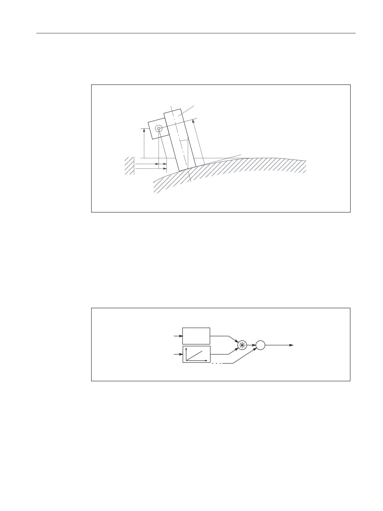
K3: Compensations
5.5 Interpolatory compensation
5.5.3.8
Example 2: Compensation with table multiplication
Compensation of sag of the foundation of a drilling machine with table multiplication.
%RULQJ PLOO
= PHDVXUHG YDOXH
=
˟
)RXQGDWLRQ XQGHU ORDG
;
ෙ;
; PHDVXUHG
YDOXH
Figure 5-15
Sag of the foundation
On large machines, sagging of the foundation can cause inclination of the whole machine.
The compensation in axis X1 depends on:
● The position of axis X1 because it determines the angle of inclination β
● The position of axis Z1, in which the drill is located.
The summed compensation value ΔX1total is calculated from the compensation values ΔX1
and ΔZ1:
ΔX1total = ΔZ1 * ΔX1 = ΔZ1 * sinβ(X1) ≈ ΔZ1 * β(X1)
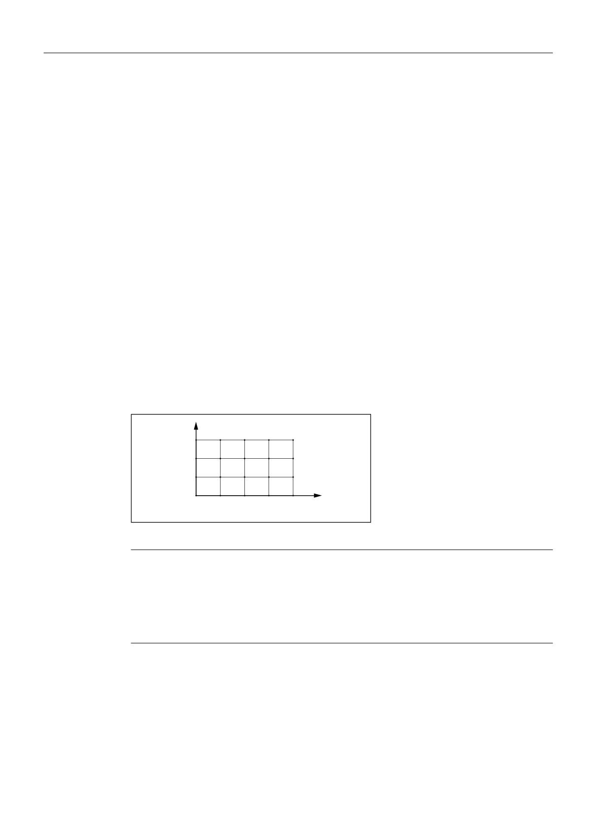
7DEOH
;
VLQ˟ ;
VHWS
ː
=
;
=
VHWS6&RPS
VHWS
;
7DEOH
Figure 5-16
Table multiplication
Compensation table 1 (table index: 0)
● Basic axis: X1
● Compensation axis: X1
● Compensation values: Sine of the position-dependent tilt angle β, with β = f(position of X1)
Extended Functions
Function Manual, 12/2018, A5E40874029B AB
297
K3: Compensations
5.5 Interpolatory compensation
Compensation table 2 (table index: 1)
● Basic axis: Z1
● Compensation axis: X1
● Compensation values: Reaction of the position of axis Z1 on the measured position of axis
X1
Table multiplication
For compensation relationship 1 (table index: 0) the table multiplication should be set with the
compensation relationship 2:
$AN_CEC_MULT_BY_TABLE[ 0 ] = 2
5.5.3.9
Example 3: 2-dimensional array of compensation values
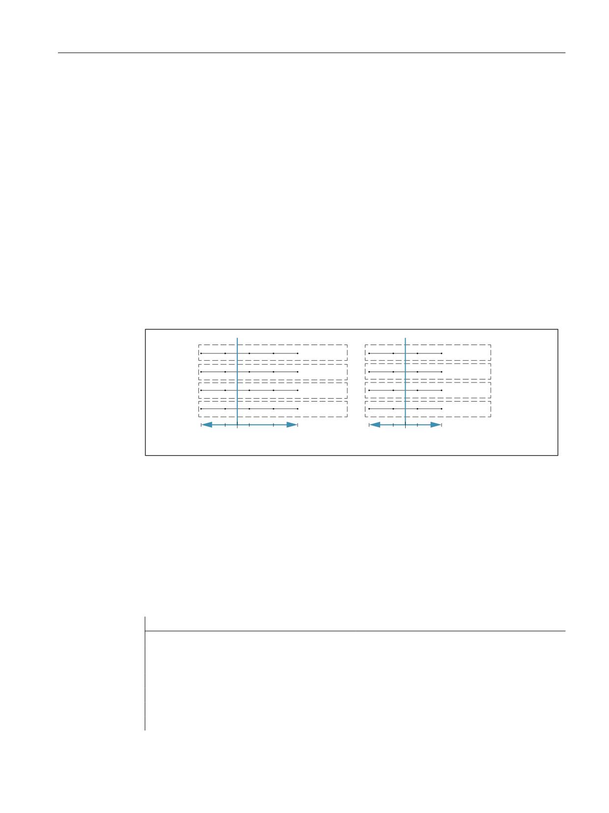
For flat-bed machines, the use case often arises in practice in which the sag compensation
values of the Z-axis depend on the axis positions of the X axis and Y axis. This is why it makes
sense to organize compensation values in a 2-dimensional array.
In this example, a possible way of implementing sag compensation using a grid, having a size
of 4 x 5 (rows x columns), is explained in more detail. The size of the complete measuring
range is 2000 x 900 mm2. The compensation values are each determined in increments of
500 mm along the X axis and 300 mm increments along the Y axis. The interpolation points
with the relevant compensation values are positioned at the intersections of the grid (X-Y
plane). Compensation values between these interpolation points are linearly interpolated.
<
;
Figure 5-17
Compensation values of the Z axis
Note
SINUMERIK Operate user interface
The currently effective compensation value of the Z axis as a result of sag compensation is
displayed on the SINUMERIK Operate user interface under:
Operating area: "Diagnostics" > "Axis diagnostics" > "Service axis" > Signal: "Compensation,
sag + temperature"
Implementation
For each line of the four-line the grid, a compensation table is set up with five interpolation
points. In the first compensation table, starting at interpolation point 1, in ascending sequence,
the compensation values 0.1 to 0.5 are entered in the first line. Using the same procedure, in
the first compensation table, compensation values 0.6 to 1.0 are entered in the second line,
Extended Functions
298
Function Manual, 12/2018, A5E40874029B AB
K3: Compensations
5.5 Interpolatory compensation
etc. These compensation tables, relevant for the position of the X axis, are now designated
with f tablesand the table values as f_i(x), with i: Table number.
Additional compensation tables are required to take into account the position of the Y axis.
These compensation tables are now designated as g tables and the table values as g_i(y).
The number of f tables and g tables is equal. In the example, four:
In the g tables, one compensation value is set to 1 - and all the others to 0. The position of
compensation value 1 within the table is determined by the table number. In the first g table,
compensation value 1 is positioned at the first interpolation point and, in the second g table,
at the second interpolation point, etc. By multiplying g tables by f tables, the correct
compensation value in each f table is selected by multiplying it by 1. All irrelevant compensation
values are concealed through multiplication by 0.
The summed compensation value Dz at position (x/y) is calculated according to the following
equation:
Dz(x/y) = f_1(x) * g_1(y) + f_2(x) * g_2(y) + f_3(x) * g_3(y) + f_4(x) * g_4(y) = k_1 + k_2 + k_3
+ k_4
At location Dz(750/450), the summed compensation value of the Z axis is calculated to be:
IB
[
JB
NB
IB
[
JB
NB
IB
[
JB
NB
IB
[
JB
NB
;
<
Dz(750/450)
= f_1(750) * g_1(450) + f_2(750) * g_2(450) +
f_3(750) * g_3(450) + f_4(750) * g_4(450)
=
0.25
*
0.0
+
0.75
*
0.5 +
1.25
*
0.5
+
1.75
*
0.0
= 1.0
Parameterization
Parameterization of machine data using the NC program
Program code
Comment
; Number of interpolation points for the compensation tables
$MN_MM_CEC_MAX_POINTS[0]=5
; Compensation table 1
$MN_MM_CEC_MAX_POINTS[1]=5
; Compensation table 2
$MN_MM_CEC_MAX_POINTS[2]=5
; Compensation table 3
$MN_MM_CEC_MAX_POINTS[3]=5
; Compensation table 4
$MN_MM_CEC_MAX_POINTS[4]=4
; Compensation table 5
$MN_MM_CEC_MAX_POINTS[5]=4
; Compensation table 6
Extended Functions
Function Manual, 12/2018, A5E40874029B AB
299

K3: Compensations
5.5 Interpolatory compensation
Program code
Comment
$MN_MM_CEC_MAX_POINTS[6]=4
; Compensation table 7
$MN_MM_CEC_MAX_POINTS[7]=4
; Compensation table 8
; Monitoring functions for axis Z1 corresponding to the 3rd machine axis
$MA_CEC_MAX_SUM[AX3]=10.0
; Max. summed compensation value
$MA_CEC_MAX_VELO[AX3]=100.0
; Max. change
Setting the table parameters (system variables) using the NC program
Program code
Comment
; To write to the compensation tables, the
; compensation for axis Z1 (compensation axis)
; must first be deactivated.
$MA_CEC_ENABLE[Z1] = FALSE
NEWCONF
; Activate $MA_CEC_ENABLE
; Define values f_i(x) in the f tables:
; Function values f_1(x) for table with index [0]
$AN_CEC[0,0]=0.1
$AN_CEC[0,1]=0.2
$AN_CEC[0,2]=0.3
$AN_CEC[0,3]=0.4
$AN_CEC[0,4]=0.5
; Function values f_2(x) for table with index [1]
$AN_CEC[1,0]=0.6
$AN_CEC[1,1]=0.7
$AN_CEC[1,2]=0.8
$AN_CEC[1,3]=0.9
$AN_CEC[1,4]=1.0
; Function values f_3(x) for table with index [2]
$AN_CEC[2,0]=1.1
$AN_CEC[2,1]=1.2
$AN_CEC[2,2]=1.3
$AN_CEC[2,3]=1.4
$AN_CEC[2,4]=1.5
; Function values f_4(x) for table with index [3]
$AN_CEC[3,0]=1.6
$AN_CEC[3,1]=1.7
$AN_CEC[3,2]=1.8
$AN_CEC[3,3]=1.9
$AN_CEC[3,4]=2.0
Extended Functions
300
Function Manual, 12/2018, A5E40874029B AB
K3: Compensations
5.5 Interpolatory compensation
Program code
Comment
; Enable evaluation of f tables with compensation values
$SN_CEC_TABLE_ENABLE[0]=TRUE
$SN_CEC_TABLE_ENABLE[1]=TRUE
$SN_CEC_TABLE_ENABLE[2]=TRUE
$SN_CEC_TABLE_ENABLE[3]=TRUE
; Define weighting factor for f tables
$SN_CEC_TABLE_WEIGHT[0]=1.0
$SN_CEC_TABLE_WEIGHT[1]=1.0
$SN_CEC_TABLE_WEIGHT[2]=1.0
$SN_CEC_TABLE_WEIGHT[3]=1.0
; Changes to the following table parameters do not take effect until
; after a warm restart
; Define basic axis X1
$AN_CEC_INPUT_AXIS[0]=(X1)
$AN_CEC_INPUT_AXIS[1]=(X1)
$AN_CEC_INPUT_AXIS[2]=(X1)
$AN_CEC_INPUT_AXIS[3]=(X1)
; Define compensation axis Z1
$AN_CEC_OUTPUT_AXIS[0]=(Z1)
$AN_CEC_OUTPUT_AXIS[1]=(Z1)
$AN_CEC_OUTPUT_AXIS[2]=(Z1)
$AN_CEC_OUTPUT_AXIS[3]=(Z1)
; Define distance between interpolation points for compensation values in f tables
$AN_CEC_STEP[0]=500.0
$AN_CEC_STEP[1]=500.0
$AN_CEC_STEP[2]=500.0
$AN_CEC_STEP[3]=500.0
; Compensation starts at X1=0
$AN_CEC_MIN[0]=0.0
$AN_CEC_MIN[1]=0.0
$AN_CEC_MIN[2]=0.0
$AN_CEC_MIN[3]=0.0
; Compensation ends at X1=2000
$AN_CEC_MAX[0]=2000.0
$AN_CEC_MAX[1]=2000.0
$AN_CEC_MAX[2]=2000.0
$AN_CEC_MAX[3]=2000.0
Extended Functions
Function Manual, 12/2018, A5E40874029B AB
301
K3: Compensations
5.5 Interpolatory compensation
Program code
Comment
; Values of f tables with index [t1] are multiplied by values in g tables
; by the number [t2]
; in accordance with the equation (algorithm) specified above
$AN_CEC_MULT_BY_TABLE[0] = 5
$AN_CEC_MULT_BY_TABLE[1] = 6
$AN_CEC_MULT_BY_TABLE[2] = 7
$AN_CEC_MULT_BY_TABLE[3] = 8
; Define the g table values for g_i(y):
; Function values g_1(x) for table with index [4]
$AN_CEC[4,0]=1.0
$AN_CEC[4,1]=0.0
$AN_CEC[4,2]=0.0
$AN_CEC[4,3]=0.0
; Function values g_2(x) for table with index [5]
$AN_CEC[5,0]=0.0
$AN_CEC[5,1]=1.0
$AN_CEC[5,2]=0.0
$AN_CEC[5,3]=0.0
; Function values g_3(x) for table with index [6]
$AN_CEC[6,0]=0.0
$AN_CEC[6,1]=0.0
$AN_CEC[6,2]=1.0
$AN_CEC[6,3]=0.0
; Function values g_4(x) for table with index [7]
$AN_CEC[7,0]=0.0
$AN_CEC[7,1]=0.0
$AN_CEC[7,2]=0.0
$AN_CEC[7,3]=1.0
; Enable evaluation of g tables with compensation values
$SN_CEC_TABLE_ENABLE[4]=TRUE
$SN_CEC_TABLE_ENABLE[5]=TRUE
$SN_CEC_TABLE_ENABLE[6]=TRUE
$SN_CEC_TABLE_ENABLE[7]=TRUE
; Define weighting factor for g tables
$SN_CEC_TABLE_WEIGHT[4]=1.0
$SN_CEC_TABLE_WEIGHT[5]=1.0
$SN_CEC_TABLE_WEIGHT[6]=1.0
$SN_CEC_TABLE_WEIGHT[7]=1.0
Extended Functions
302
Function Manual, 12/2018, A5E40874029B AB
K3: Compensations
5.5 Interpolatory compensation
Program code
Comment
; Changes to the following table parameters do not take effect until
; a power on is carried out
;Define basic axis Y1
$AN_CEC_INPUT_AXIS[4]=(Y1)
$AN_CEC_INPUT_AXIS[5]=(Y1)
$AN_CEC_INPUT_AXIS[6]=(Y1)
$AN_CEC_INPUT_AXIS[7]=(Y1)
; Define compensation axis Z1
$AN_CEC_OUTPUT_AXIS[4]=(Z1)
$AN_CEC_OUTPUT_AXIS[5]=(Z1)
$AN_CEC_OUTPUT_AXIS[6]=(Z1)
$AN_CEC_OUTPUT_AXIS[7]=(Z1)
; Define distance between interpolation points for compensation values in g tables
$AN_CEC_STEP[4]=300.0
$AN_CEC_STEP[5]=300.0
$AN_CEC_STEP[6]=300.0
$AN_CEC_STEP[7]=300.0
;Compensation starts at Y1=0
$AN_CEC_MIN[4]=0.0
$AN_CEC_MIN[5]=0.0
$AN_CEC_MIN[6]=0.0
$AN_CEC_MIN[7]=0.0
;Compensation ends at Y1=900
$AN_CEC_MAX[4]=900.0
$AN_CEC_MAX[5]=900.0
$AN_CEC_MAX[6]=900.0
$AN_CEC_MAX[7]=900.0
; Activate compensation again
$MA_CEC_ENABLE[Z1]=TRUE
NEWCONF
; Carry out a program test to check that the compensation is active
G01 F1000 X0 X0 Z0 G90
R1=0 R2=0
LOOP_Y:
LOOP_X:
STOPRE
X=R1 Y=R2
M0
; Wait to check the CEC value
Extended Functions
Function Manual, 12/2018, A5E40874029B AB
303
K3: Compensations
5.5 Interpolatory compensation
Program code
Comment
R1=R1+500
IF R1 <=2000 GOTOB LOOP_X
R1=0
R2=R2+300
IF R2<=900 GOTOB LOOP_Y
5.5.4
Extension of the sag compensation with NCU link - only 840D sl
5.5.4.1
General parameter assignment
Basic and compensation axes
The parameterization of the basic axis (input) and compensation axis (output) of a
compensation table is realized in conjunction with link axes (Page 80) using the following
system variables:
● $AN_CEC_INPUT_NCU
● $AN_CEC_INPUT_AXIS
● $AN_CEC_OUTPUT_NCU
● $AN_CEC_OUTPUT_AXIS
The following supplementary conditions must be observed:
● The basic and compensation axes of the sag compensation must be interpolated as channel
axes on the same NCU.
● The corresponding machine axes can be connected to different NCUs.
● The system variables become effective only after a warm restart of the NCU.
● Data backup is undertaken with machine axis names.
General commissioning of the sag compensation
For general commissioning of the sag compensation, see Chapter "Commissioning: Basic
procedure (Page 293)".
5.5.4.2
Parameterization with channel names
The parameterization of basic and compensation axes with channel axis names takes place
with the following system variables:
● Input axis
$AN_CEC_INPUT_AXIS[<CEC table number>] = <channel axis name>
● Output axis
$AN_CEC_OUTPUT_AXIS[<CEC table number>] = <channel axis name>
Extended Functions
304
Function Manual, 12/2018, A5E40874029B AB
K3: Compensations
5.5 Interpolatory compensation
Example: Coupling axis "ZZ" (AX2, NCU 2) to "XR" (AX1, NCU 1)
Two part programs, TP1 for channel 1 and TP2 for channel 2, have to be created. The system
variables of the basic and compensation axes of the compensation table are written to these.
Excerpt from TP1, channel 1: $AN_CEC_INPUT_AXIS[0] = "XR"
Excerpt from TP2, channel 2: $AN_CEC_OUTPUT_AXIS[0] = "ZZ"
5.5.4.3
Parameterization with machine axis names
The parameterization of basic and compensation axes with machine axis names takes place
with the following system variables:
● Basic axis
- $AN_CEC_INPUT_NCU[<CEC table number>] = <NCU number>
- $AN_CEC_INPUT_AXIS[<CEC table number>] = <machine axis name>
● Compensation axes
- $AN_CEC_OUTPUT_NCU[<CEC table number>] = <NCU number>
- $AN_CEC_OUTPUT_AXIS[<CEC table number>] = <channel axis name>
Example: Coupling axis "ZZ" (AX2, NCU 2) to "XR" (AX1, NCU 1)
A part program has to be created, which can be started in any channel of the NCU 1. The
system variables of the basic and compensation axes of the compensation table with machine
axis names and NCU number are written to these.
Part program:
$AN_CEC_INPUT_NCU[0] = 1
$AN_CEC_INPUT_AXIS[0] = "AX1"
$AN_CEC_OUTPUT_NCU[0] = 2
$AN_CEC_OUTPUT_AXIS[0] = "AX2"
Note
● The NCU number must be written to the NC program before the axis names.
● Sag compensation between NC1_AX1 and NC2_AX2 is not possible.
5.5.4.4
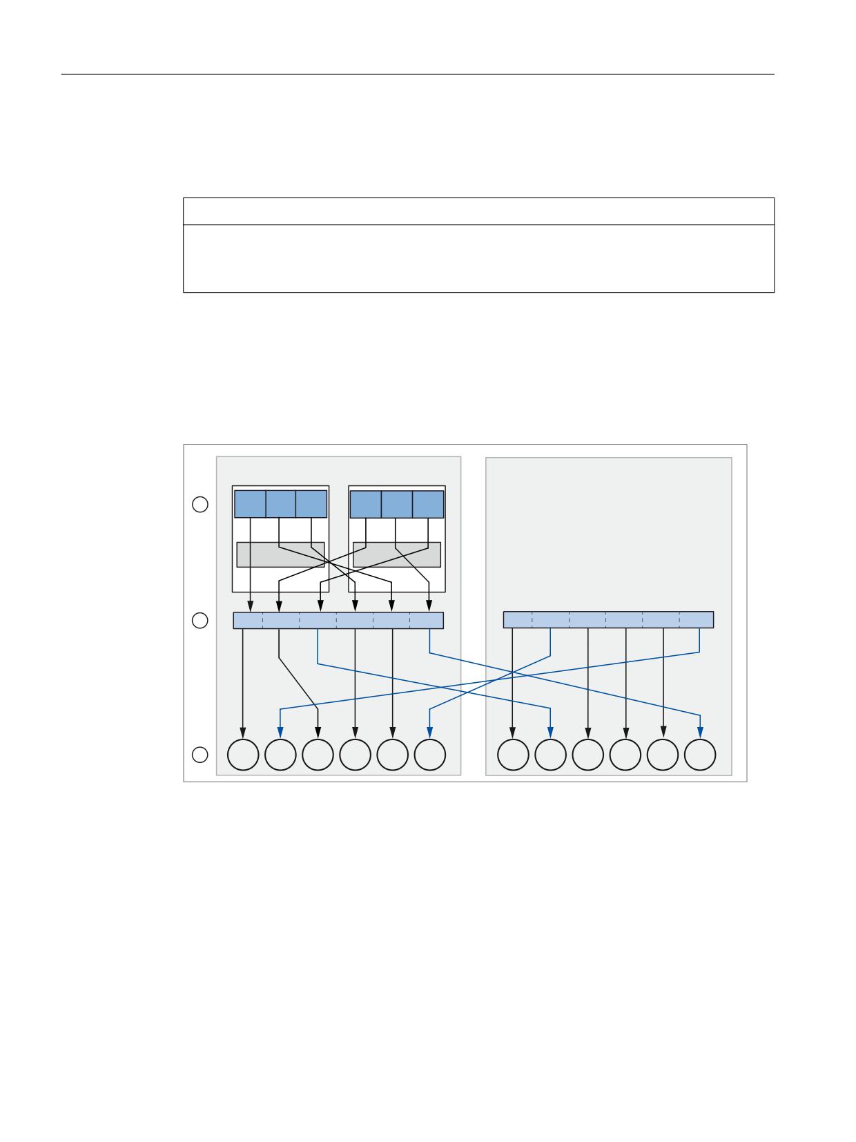
Axis container
Sag compensation can also be used in conjunction with container axes (Page 101). It should
be noted that when using container axes, after each axis container rotation, other machine
axes are coupled regarding sag compensation. In order to maintain the coupling between two
specific machine axes, even after an axis container rotation, after each rotation, the system
variables to parameterize the basic and compensation axes must be appropriately newly
written to the compensation table by the user.
Extended Functions
Function Manual, 12/2018, A5E40874029B AB
305
K3: Compensations
5.5 Interpolatory compensation
Requirement
The axis container has to be located in the start position ($AN_AXCTAS == 0) when the sag
compensation is activated.
NOTICE
Changing the machine axes
After a axis container rotation, the same channel axes remain coupled. The coupled machine
axes can change.
5.5.4.5
Configuration example 1: NCU link with rigid coupling
In configuration example 1, the two channels of NCU 1 - and the channel axis names defined
using machine data MD20080 $MC_AXCONF_CHANAX_NAME_TAB - are shown. The
configuration of NCU 2 is not shown.
1&8
1&8
&KDQQHO
&KDQQHO
;5
<5
=5
;;
<<
==
,QWHUSRODWLRQ
,QWHUSRODWLRQ
$;
$;
$;
$;
$;
$;
$;
$;
$;
$;
$;
$;
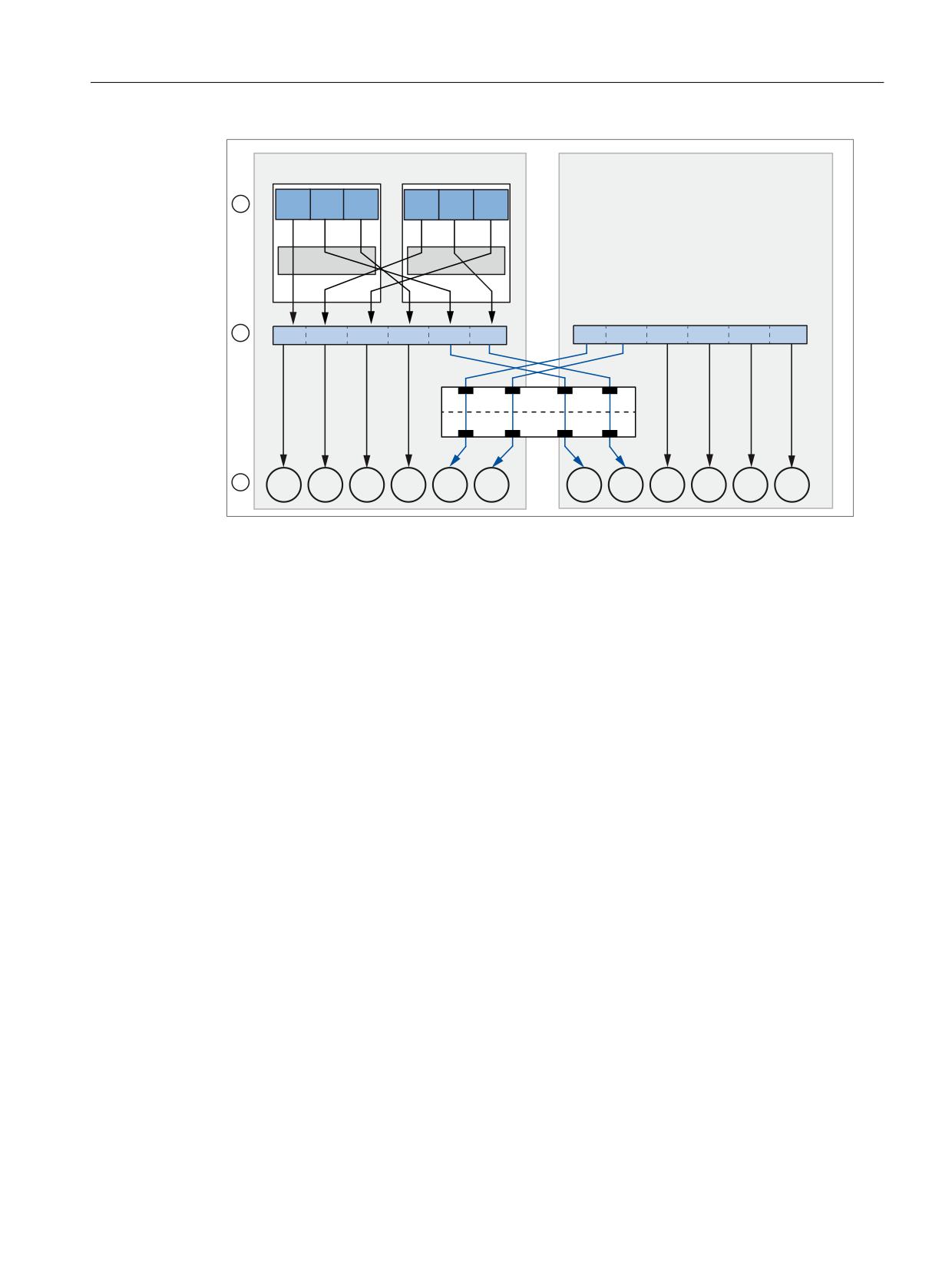
① Assignment of channel axes to machine axes:
MD20070 $MC_AXCONF_MACHAX_USED[0 ... 2]
② Assignment of logical to real machine axes:
MD10002 $MN_AXCONF_LOGIC_MACHAX_TAB
③ Machine axis names:
MD10000 $MN_AXCONF_MACHAX_NAME_TAB
Figure 5-18
Configuration 1: NCU link with rigid coupling
Channel axis ZZ (NCU1, channel 2) is connected to machine axis AX2 of NCU 2. This means
that in order that machine axis AX2 of NCU 2 traverses, in the 2nd channel of NCU 1, axis ZZ
is traversed. For example, using the following commands in an NC program:
POS[ZZ]=10 FA[ZZ]=1000
Extended Functions
306
Function Manual, 12/2018, A5E40874029B AB
K3: Compensations
5.5 Interpolatory compensation
Parameterization
The machine data of both NCUs is parameterized using the subsequently listed NC programs
NC_P1 and NC_P2.
NC program NC_P1: Parameterization of the machine data for NCU 1
Program code
; ########## NCU1 ##########
; NC-specific machine data
$MN_NCU_LINKNO = 1
$MN_MM_NCU_LINK_MASK = 1
$MN_MM_LINK_NUM_OF_MODULES= 2
$MN_MM_SERVO_FIFO_SIZE = 3
$MN_ASSIGN_CHAN_TO_MODE_GROUP[1]=1
$MN_AXCONF_LOGIC_MACHAX_TAB[0] = "NC1_AX1"
$MN_AXCONF_LOGIC_MACHAX_TAB[1] = "NC1_AX3"
$MN_AXCONF_LOGIC_MACHAX_TAB[2] = "NC2_AX2"
$MN_AXCONF_LOGIC_MACHAX_TAB[3] = "NC1_AX4"
$MN_AXCONF_LOGIC_MACHAX_TAB[4] = "NC1_AX5"
$MN_AXCONF_LOGIC_MACHAX_TAB[5] = "NC2_AX6"
; Channel-specific machine data: Channel 1
CHANDATA(1)
$MC_AXCONF_MACHAX_USED[0]=1
$MC_AXCONF_MACHAX_USED[1]=5
$MC_AXCONF_MACHAX_USED[2]=4
$MC_AXCONF_MACHAX_USED[3]=0
$MC_AXCONF_MACHAX_USED[4]=0
$MC_AXCONF_MACHAX_USED[5]=0
$MC_AXCONF_CHANAX_NAME_TAB[0] = "XR"
$MC_AXCONF_CHANAX_NAME_TAB[1] = "YR"
$MC_AXCONF_CHANAX_NAME_TAB[2] = "ZR"
; Channel-specific machine data: Channel 2
CHANDATA(2)
$MC_REFP_NC_START_LOCK=0
$MC_AXCONF_MACHAX_USED[0]=2
$MC_AXCONF_MACHAX_USED[1]=6
$MC_AXCONF_MACHAX_USED[2]=3
$MC_AXCONF_MACHAX_USED[3]=0
$MC_AXCONF_MACHAX_USED[4]=0
$MC_AXCONF_MACHAX_USED[5]=0
$MC_AXCONF_CHANAX_NAME_TAB[0] = "XX"
$MC_AXCONF_CHANAX_NAME_TAB[1] = "YY"
$MC_AXCONF_CHANAX_NAME_TAB[2] = "ZZ"
M30
Extended Functions
Function Manual, 12/2018, A5E40874029B AB
307
K3: Compensations
5.5 Interpolatory compensation
NC program NC_P2: Parameterization of machine data for NCU 2
Program code
; ########## NCU-2 ##########
; NC-specific machine data
$MN_NCU_LINKNO = 2
$MN_MM_NCU_LINK_MASK = 1
$MN_MM_LINK_NUM_OF_MODULES= 2
$MN_MM_SERVO_FIFO_SIZE = 3
$MN_AXCONF_LOGIC_MACHAX_TAB[0] = "NC2_AX1"
$MN_AXCONF_LOGIC_MACHAX_TAB[1] = "NC1_AX6"
$MN_AXCONF_LOGIC_MACHAX_TAB[2] = "NC2_AX3"
$MN_AXCONF_LOGIC_MACHAX_TAB[3] = "NC2_AX4"
$MN_AXCONF_LOGIC_MACHAX_TAB[4] = "NC2_AX5"
$MN_AXCONF_LOGIC_MACHAX_TAB[5] = "NC1_AX2"
; Channel-specific machine data: Channel 1
CHANDATA(1)
$MC_AXCONF_MACHAX_USED[0]=1
$MC_AXCONF_MACHAX_USED[1]=2
$MC_AXCONF_MACHAX_USED[2]=3
$MC_AXCONF_MACHAX_USED[3]=4
$MC_AXCONF_MACHAX_USED[4]=5
$MC_AXCONF_MACHAX_USED[5]=6
$MC_AXCONF_MACHAX_USED[6]=0
M30
5.5.4.6
Configuration example 2 NCU link with axis container
Configuration example 2 contains an axis container (Page 101) CT1. The parameterization of
the axes contained in the axis container is realized using MD12701
$MN_AXCT_AXCONF_ASSIGN_TAB1. The axis container is a multi-NCU object that only
exists once for all NCUs.
The logical machine axis of channel axis YR refers to slot CT1_SL3 - and channel axis YY to
slot CT1_SL4. The channel axes of NCU2 are not shown.
Container axes are assigned to the following machine axes:
● NC1_AX5
● NC1_AX6
● NC2_AX1
● NC2_AX2
Axis constellation in the initial state of the axis container
In the initial state of the axis container, after the NCUs power up, channel axis YR is connected
with NC2_AX1 and channel axis YY with NC2_AX2.
Extended Functions
308
Function Manual, 12/2018, A5E40874029B AB
K3: Compensations
5.5 Interpolatory compensation
1&8
1&8
.DQDO
DQDO
;5
<5
=5
;;
<<
==
,QWHUSRODWLRQ
,QWHUSRODWLRQ
$[LV
FRQWDLQHU
$;
$;
$;
$;
$;
$;
$;
$;
$;
$;
$;
$;
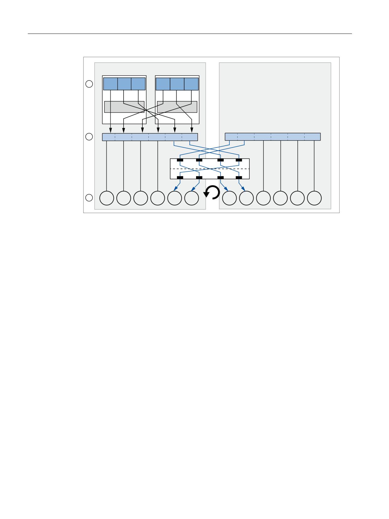
① MD20070 $MC_AXCONF_MACHAX_USED.
② MD10002 $MN_AXCONF_LOGIC_MACHAX_TAB
③ MD10000 $MN_AXCONF_MACHAX_NAME_TAB
Axis constellation after one axis container step
After the axis container rotates through one step (increment), channel axis YR is connected
to NC2_AX2, and channel axis YY is connected to NC1_AX5.
Extended Functions
Function Manual, 12/2018, A5E40874029B AB
309
K3: Compensations
5.5 Interpolatory compensation
1&8
1&8
&KDQQHO
&KDQQHO
;5
<5
=5
;;
<<
==
,QWHUSRODWLRQ
,QWHUSRODWLRQ
$[LV FRQWDLQHU
$;
$;
$;
$;
$;
$;
$;
$;
$;
$;
$;
$;
① MD20070 $MC_AXCONF_MACHAX_USED.
② MD10002 $MN_AXCONF_LOGIC_MACHAX_TAB
③ MD10000 $MN_AXCONF_MACHAX_NAME_TAB
NC program NC_P1: Parameterization of the machine data for NCU 1
Program code
; ########## NCU1 ##########
; NC-specific machine data
$MN_NCU_LINKNO = 1
$MN_MM_NCU_LINK_MASK = 1
$MN_MM_LINK_NUM_OF_MODULES= 2
$MN_MM_SERVO_FIFO_SIZE = 3
$MN_ASSIGN_CHAN_TO_MODE_GROUP[1]=1
$MN_AXCONF_LOGIC_MACHAX_TAB[0] = "NC1_AX1"
$MN_AXCONF_LOGIC_MACHAX_TAB[1] = "NC1_AX3"
$MN_AXCONF_LOGIC_MACHAX_TAB[2] = "NC2_AX2"
$MN_AXCONF_LOGIC_MACHAX_TAB[3] = "NC1_AX4"
$MN_AXCONF_LOGIC_MACHAX_TAB[4] = "CT1_SL3"
$MN_AXCONF_LOGIC_MACHAX_TAB[5] = "CT1_SL4"
$MN_AXCT_AXCONF_ASSIGN_TAB1[0] = "NC1_AX5"
$MN_AXCT_AXCONF_ASSIGN_TAB1[1] = "NC1_AX6"
$MN_AXCT_AXCONF_ASSIGN_TAB1[2] = "NC2_AX1"
$MN_AXCT_AXCONF_ASSIGN_TAB1[3] = "NC2_AX2"
$SN_AXCT_SWWIDTH[0] = 1
; Channel-specific machine data: Channel 1
CHANDATA(1)
Extended Functions
310
Function Manual, 12/2018, A5E40874029B AB
K3: Compensations
5.5 Interpolatory compensation
Program code
$MC_AXCONF_MACHAX_USED[0]=1
$MC_AXCONF_MACHAX_USED[1]=5
$MC_AXCONF_MACHAX_USED[2]=4
$MC_AXCONF_MACHAX_USED[3]=0
$MC_AXCONF_MACHAX_USED[4]=0
$MC_AXCONF_MACHAX_USED[5]=0
$MC_AXCONF_CHANAX_NAME_TAB[0] = "XR"
$MC_AXCONF_CHANAX_NAME_TAB[1] = "YR"
$MC_AXCONF_CHANAX_NAME_TAB[2] = "ZR"
; Channel-specific machine data: Channel 1
CHANDATA(2)
$MC_REFP_NC_START_LOCK=0
$MC_AXCONF_MACHAX_USED[0]=2
$MC_AXCONF_MACHAX_USED[1]=6
$MC_AXCONF_MACHAX_USED[2]=3
$MC_AXCONF_MACHAX_USED[3]=0
$MC_AXCONF_MACHAX_USED[4]=0
$MC_AXCONF_MACHAX_USED[5]=0
$MC_AXCONF_CHANAX_NAME_TAB[0] = "XX"
$MC_AXCONF_CHANAX_NAME_TAB[1] = "YY"
$MC_AXCONF_CHANAX_NAME_TAB[2] = "ZZ"
M30
NC program NC_P2: Parameterization of machine data for NCU 2
Program code
; ########## NCU-2 ##########
; NC-specific machine data
$MN_NCU_LINKNO = 2
$MN_MM_NCU_LINK_MASK = 1
$MN_MM_LINK_NUM_OF_MODULES= 2
$MN_MM_SERVO_FIFO_SIZE = 3
$MN_AXCONF_LOGIC_MACHAX_TAB[0] = "CT1_SL1"
$MN_AXCONF_LOGIC_MACHAX_TAB[1] = "CT1_SL2"
$MN_AXCONF_LOGIC_MACHAX_TAB[2] = "NC2_AX3"
$MN_AXCONF_LOGIC_MACHAX_TAB[3] = "NC2_AX4"
$MN_AXCONF_LOGIC_MACHAX_TAB[4] = "NC2_AX5"
$MN_AXCONF_LOGIC_MACHAX_TAB[5] = "NC2_AX6"
CHANDATA(1)
; Channel-specific machine data: Channel 1
$MC_AXCONF_MACHAX_USED[0]=1
$MC_AXCONF_MACHAX_USED[1]=2
$MC_AXCONF_MACHAX_USED[2]=3
$MC_AXCONF_MACHAX_USED[3]=4
Extended Functions
Function Manual, 12/2018, A5E40874029B AB
311
K3: Compensations
5.5 Interpolatory compensation
Program code
$MC_AXCONF_MACHAX_USED[4]=5
$MC_AXCONF_MACHAX_USED[5]=6
$MC_AXCONF_MACHAX_USED[6]=0
M30
5.5.5
Direction-dependent leadscrew error compensation
5.5.5.1
Description of functions
If the direction-dependent differences at the compensation points are excessively high, for an
inconsistent backlash or for extremely high demands placed on the precision, then it may be
necessary to apply direction-dependent compensation of the leadscrew error or measuring
system error (for direct position sensing).
Direction-dependent leadscrew error compensation
For the "direction-dependent leadscrew error compensation" ("direction-dependent LEC" or
also "Bidirectional LEC") , two compensation tables are used for each axis. One compensation
table for the positive and one compensation table for the negative traversing direction. The
deviation at the particular compensation point is entered as difference between the ideal
setpoint and measured actual value in the compensation tables. The control automatically
calculates compensation values of intermediate values using linear interpolation.
Preconditions / activation
The "direction-dependent LEC" is implemented in the SINUMERIK control as a special case
of "sag compensation". This is the reason that the preconditions and conditions of "sag
compensation" apply (see "Sag and angularity error compensation (Page 285)").
The activation of the compensation can be checked using a reference measurement, e.g. using
the laser interferometer or in the simplest case, using the service display of the particular axis.
Note
If the "direction-dependent LEC" is used in parallel to the sag compensation and compensation
of the angularity, then the secondary conditions of these functions must be taken into
consideration together, e.g. the assignment of tables <t> to the particular function.
Extended Functions
312
Function Manual, 12/2018, A5E40874029B AB
K3: Compensations
5.5 Interpolatory compensation
5.5.5.2
Commissioning
Measuring the error or compensation values
When commissioning the "direction-dependent LEC" - just the same as when commissioning
the "direction-dependent LEC" - direction-dependent error curves for each axis are determined
using a suitable measuring device (e.g. laser interferometer) (see Section "Leadscrew error
and measuring system error compensation (Page 280)"). A part program with measurement
points and wait times should be generated in order to perform the measurement (see Section
"Example (Page 316)"): Program "BI_SSFK_MESS_AX1_X.MPF").
Because the various measuring devices offer different support options for the practical
implementation in conjunction with a SINUMERIK control, this process is only generally
described in the following referred to a control.
Note
The measurement for determining the leadscrew error should only be carried out during the
first commissioning if, in the machine data, the traversing directions of the axes in relation to
the machine coordinate system have been correctly set.
Extended Functions
Function Manual, 12/2018, A5E40874029B AB
313
K3: Compensations
5.5 Interpolatory compensation
Commissioning (principle)
1.
Specify the number of compensation interpolation points (also see Section "Compensation
for droop and angularity error: Commissioning (Page 293)")
For the directional leadscrew error compensation, a compensation table for the positive
and a compensation table for the negative traversing directions must be assigned to each
axis. The number of compensation interpolation points of a table is defined in:
MD18342 $MN_MM_CEC_MAX_POINTS[ <compensation table index> ]
CAUTION
Possible data loss
A change to the machine data MD18342 $MN_MM_CEC_MAX_POINTS, which
configures memory, reconfigures (Page 829) the NC memory the next time the control
starts. This can result in the loss of all user-specific data.
Creating a commissioning archive:
Operating area: "Commissioning" > "ETC" key > "Commissioning archive" > "Create
commissioning archive" > "OK" > Selection: "NC data"
Example
- X axis: positive traversing direction, table 1, 11 interpolation points
- X axis: negative traversing direction, table 2, 11 interpolation points
Machine data:
- MD18342 $MN_MM_CEC_MAX_POINTS[ 0 ] = 11
- MD18342 $MN_MM_CEC_MAX_POINTS[ 1 ] = 11
2.
Reading in a commissioning archive that has been created:
Operating area: "Commissioning" > "ETC" key > "Commissioning archive" > "Read in
commissioning archive" > "OK"
The compensation tables are then available.
3.
To simplify commissioning, create an NC program by which the compensation parameters
are written into the machine data and system variables (see Section "Example (Page 316)").
4.
Run the NC program on the control:
Mode: "AUTOMATIC" > Select program > NC start
5.
Power-on (warm restart).
6.
Now, comparative measurements can be made using the laser interferometer.
7.
To further improve the compensation results, it is also conceivable to correct individual
compensation values in the program. A POWER ON is no longer necessary when reading-
in the table again.
Extended Functions
314
Function Manual, 12/2018, A5E40874029B AB

K3: Compensations
5.5 Interpolatory compensation
Note
Sequence for SINUMERIK 828D
For SINUMERIK 828D, steps 2 and 3 are eliminated. This is because when the "sag
compensation, multi-dimensional" option is enabled, 12 tables each with 200 interpolation
points per table for the compensation immediately become available. This cannot be extended!
NC_CEC.INI
The "NC_CEC.INI" file copied via "Commissioning" > "System data" (from the folder "NC active
data" > "sag angularity comp") includes all negotiated sag/angularity and direction-dependent
LEC tables.
Backlash
The backlash should be set to 0:
● MD32450 $MA_BACKLASH [ <measuring system> ] = 0
Compensation parameters
The compensation parameters are set via the following system variables:
● $AN_CEC[ <table>,<interpolation point> ] (compensation value)
● $AN_CEC_INPUT_AXIS[ <table> ] (basic axis)
● $AN_CEC_OUTPUT_AXIS[ <table> ] (compensation axis)
Note
For the "directional LEC," the basis and compensation axes are alwaysidentical.
● $AN_CEC_STEP[ <table> ] (distance between interpolation points)
● $AN_CEC_MIN[ <table> ] (starting position)
● $AN_CEC_MAX[ <table> ] (end position)
● $AN_CEC_DIRECTION[ <table> ] (direction)
Note
The setting $AN_CEC_DIRECTION[<t>] = 0 (table is effective for both traversing directions
of the basic axis) is not relevant for the "direction-dependent LEC".
● $AN_CEC_IS_MODULO[ <table> ] (compensation with modulo function)
Note
For a description of these system variables, see Section "Compensation of sag and angularity
error: commissioning (Page 293)".
Extended Functions
Function Manual, 12/2018, A5E40874029B AB
315

K3: Compensations
5.5 Interpolatory compensation
System of units
See Section "Compensation for droop and angularity error: Commissioning (Page 293)".
Monitoring
See Section "Compensation for droop and angularity error: Commissioning (Page 293)".
5.5.5.3
Example
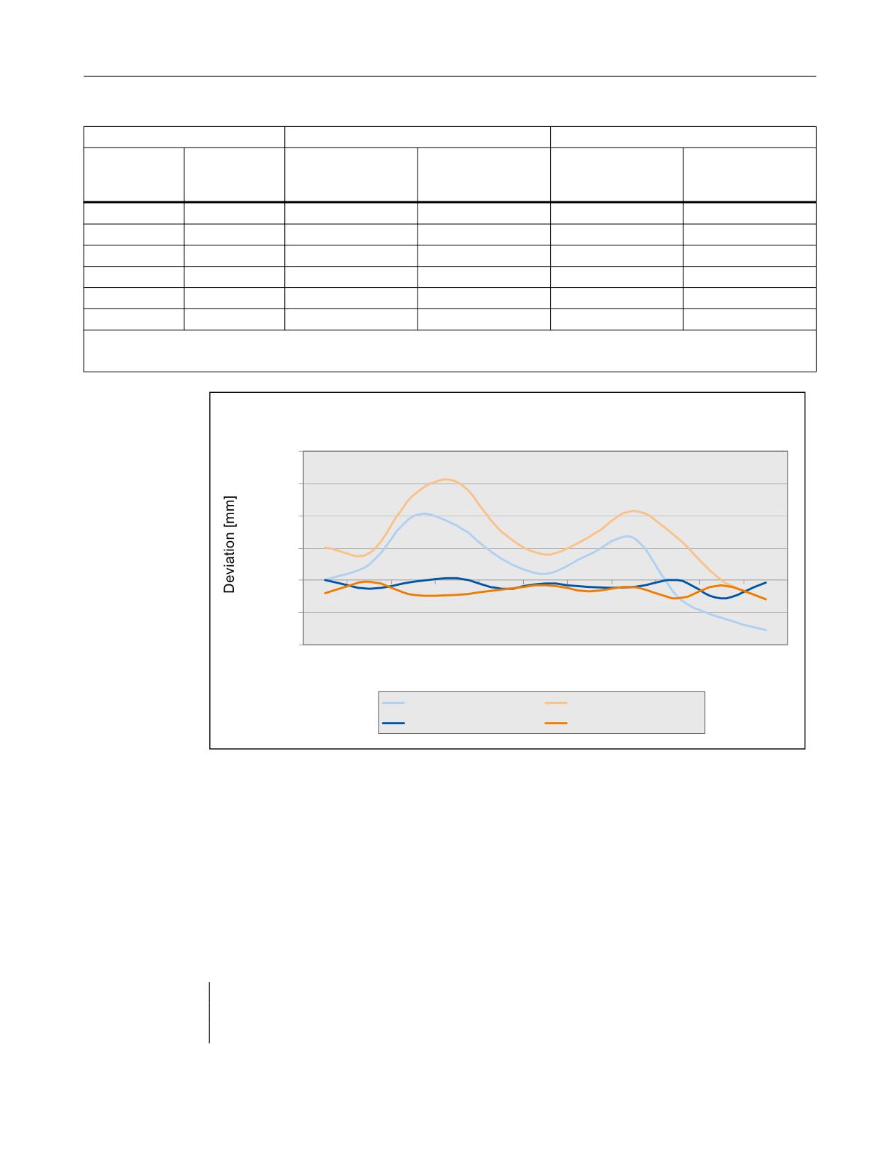
The following examples shows parameterization of the directional compensation tables for an
axis (machine axis AX1). All parameter values of the compensation tables are written by means
of a program.
Compensation parameters
● Basic axis = compensation axis = machine axis AX1
● Distance between interpolation points: 58.0 mm
● Starting position: -585.0 mm
● End position: -5.0 mm
Table definition
The 1st and 2nd compensation table are defined with 11 compensation interpolation points
each for machine axis AX1 as directional compensation tables:
● MD18342 $MN_MM_CEC_MAX_POINTS[ 0 ] = 11 (table 1: positive traversing direction)
● MD18342 $MN_MM_CEC_MAX_POINTS[ 1 ] = 11 (table 2: negative traverse direction)
Note
It is not necessary to define the number of interpolation points for SINUMERIK 828D, because
when enabling the "sag compensation, multi-dimensional" option, immediately 12 tables each
with 200 interpolation points per table for the compensation are available. This cannot be
extended!
Interpolation points and correction values
Interpolation points
Deviations or correction values
Deviation with compensation
Index
Position
pos. Traversing di-
neg. Traversing di-
pos. Traversing di-
neg. Traversing di-
[mm]
rection
rection
rection
rection
[mm]
[mm]
[mm]
[mm]
0
-585 1)
0.0000
0.0020
0.0000
-0.0008
1
-527
0.0010
0.0017
-0.0005
-0.0001
2
-469
0.0040
0.0053
-0.0001
-0.0009
3
-411
0.0034
0.0061
0.0001
-0.0009
4
-353
0.0013
0.0030
-0.0005
-0.0006
Extended Functions
316
Function Manual, 12/2018, A5E40874029B AB
K3: Compensations
5.5 Interpolatory compensation
Interpolation points
Deviations or correction values
Deviation with compensation
Index
Position
pos. Traversing di-
neg. Traversing di-
pos. Traversing di-
neg. Traversing di-
[mm]
rection
rection
rection
rection
[mm]
[mm]
[mm]
[mm]
5
-295
0.0004
0.0016
-0.0002
-0.0003
6
-237
0.0016
0.0027
-0.0004
-0.0007
7
-179
0.0026
0.0043
-0.0004
-0.0004
8
-121
-0.0010
0.0026
0.0000
-0.0011
9
-63
-0.0023
0.0000
-0.0011
-0.0003
10
-5 2)
-0.0031
-0.0012
-0.0001
-0.0012
1) Starting position: $AC_CEC_MIN[ <Table> ]
2) End position: $AC_CEC_MAX[ <Table> ]
(UURU FXUYH ; D[LV
3RVLWLRQ ;
; ZLWKRXW FRPSHQVDWLRQ
; ZLWKRXW FRPSHQVDWLRQ
; ZLWK FRPSHQVDWLRQ
; ZLWK FRPSHQVDWLRQ
Programming
The following actions are performed by program "BI_SSFK_TAB_AX1_X.MPF":
● Deactivation of the compensation
● Deactivation of the compensation tables to be written (active tables cannot be written).
● Writing the compensation values into the compensation tables for the positive and negative
traversing direction of the X axis
● Writing the compensation parameters
; directional LEC
; 1st axis AX1
; table 1 - positive traversing direction
Extended Functions
Function Manual, 12/2018, A5E40874029B AB
317
K3: Compensations
5.5 Interpolatory compensation
; table 2 - negative traversing direction
;--- Deaktivierung der Kompensation und der Tabellen
CHANDATA(1)
$MA_CEC_ENABLE[AX1]=0
; compensation OFF
$SN_CEC_TABLE_ENABLE[0]=0
; lock Table 1
$SN_CEC_TABLE_ENABLE[1]=0
; lock Table 2
NEWCONF
;--- 1. Kompensationstabelle, positive Verfahrrichtung
;------ Kompensationswerte
$AN_CEC[0,0]=0
; correction value interpolation point 0
$AN_CEC[0,1]=0.001
; correction value interpolation point 1
$AN_CEC[0,2]=0.004
; correction value interpolation point 2
$AN_CEC[0,3]=0.0034
; correction value interpolation point 3
$AN_CEC[0,4]=0.0013
; correction value interpolation point 4
$AN_CEC[0,5]=0.0004
; correction value interpolation point 5
$AN_CEC[0,6]=0.0016
; correction value interpolation point 6
$AN_CEC[0,7]=0.0026
; correction value interpolation point 7
$AN_CEC[0,8]=-0.001
; correction value interpolation point 8
$AN_CEC[0,9]=-0.0023
; correction value interpolation point 9
$AN_CEC[0,10]=-0.0031
; correction value interpolation point 10
; ------ Kompensationsparame-
ter
$AN_CEC_INPUT_AXIS[0]=(AX1)
; basic axis
$AN_CEC_OUTPUT_AXIS[0]=(AX1)
; compensation axis
$AN_CEC_STEP[0]=58.0
; distance between interpolation points
$AN_CEC_MIN[0]=-585.0
; starting position
$AN_CEC_MAX[0]=-5.0
; end position
$AN_CEC_DIRECTION[0]=1
; table applies to positive traversing directions
$AN_CEC_MULT_BY_TABLE[0]=0
; no multiplication (not relevant here)
$AN_CEC_IS_MODULO[0]=0
; compensation without modulo function
;--- 2. Kompensationstabelle, negative Verfahrrichtung
;------ Kompensationswerte
$AN_CEC[1,0]=0.002
; correction value interpolation point 0
$AN_CEC[1,1]=0.0017
; correction value interpolation point 1
$AN_CEC[1,2]=0.0053
; correction value interpolation point 2
$AN_CEC[1,3]=0.0061
; correction value interpolation point 3
$AN_CEC[1,4]=0.003
; correction value interpolation point 4
$AN_CEC[1,5]=0.0016
; correction value interpolation point 5
$AN_CEC[1,6]=0.0027
; correction value interpolation point 6
$AN_CEC[1,7]=0.0043
; correction value interpolation point 7
$AN_CEC[1,8]=0.0026
; correction value interpolation point 8
$AN_CEC[1,9]=0.000
; correction value interpolation point 9
$AN_CEC[1,10]=-0.0012
; correction value interpolation point 10
; ------ Kompensationsparame-
ter
$AN_CEC_INPUT_AXIS[1]=(AX1)
; basic axis
Extended Functions
318
Function Manual, 12/2018, A5E40874029B AB
K3: Compensations
5.5 Interpolatory compensation
$AN_CEC_OUTPUT_AXIS[1]=(AX1)
; compensation axis
$AN_CEC_STEP[1]=58.0
; distance between interpolation points
$AN_CEC_MIN[1]=-585.0
; starting position
$AN_CEC_MAX[1]=-5.0
; end position
$AN_CEC_DIRECTION[1]=-1
; table applies to negative traversing directions
$AN_CEC_MULT_BY_TABLE[1]=0
; no multiplication (not relevant here)
$AN_CEC_IS_MODULO[1]=0
; compensation without modulo function (for rotary
axes only)
;--- Aktivierung der Kompensation und der Tabellen
$MA_CEC_ENABLE[AX1]=1
; compensation ON
$SN_CEC_TABLE_ENABLE[0]=1
; enable table 1
$SN_CEC_TABLE_ENABLE[1]=1
; enable table 2
NEWCONF
M17
; end of program
5.5.6
Cylinder error compensation
5.5.6.1
Options
The following option is required to use the "Cylindrical error compensation" function:
● SINUMERIK Grinding Advanced (6FC5800-0AS35-0YB0)
5.5.6.2
Function
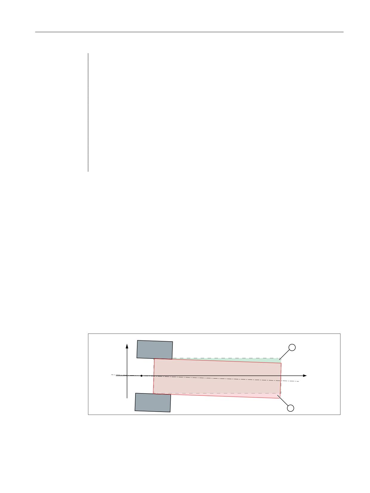
The cylinder error compensation is used to compensate for clamping errors for cylindrical
grinding. In this case, a shift and/or rotation of the workpiece in the machining plane is
compensated.
Contrary to Sag and angularity error compensation (Page 285), which is used as basis for
cylinder error compensation, only two interpolation points are used to define the compensation
function (straight line).
;
=
① Set position of the cylinder
② Actual position of the cylinder
Figure 5-19
Cylinder error due to incorrect clamping
Extended Functions
Function Manual, 12/2018, A5E40874029B AB
319

K3: Compensations
5.5 Interpolatory compensation
5.5.6.3
Commissioning
Number
Identifier
Meaning
SD41300
$SN_CEC_TABLE_ENABLE
Compensation table enable
SD41310
$SN_CEC_TABLE_WEIGHT
Weighting factor
SD41320
$SN_CEC_0
Compensation value at the starting position
SD41321
$SN_CEC_1
Compensation value at the end position
SD41330
$SN_CEC_BAS_0
Measuring point P1: Basic value
SD41331
$SN_CEC_BAS_1
Measuring point P2: Basic value
SD41335
$SN_CEC_BAS_STORE_0
Bit memories for measuring point P1: Basic value
SD41336
$SN_CEC_BAS_STORE_1
Bit memories for measuring point P2: Basic value
SD41340
$SN_CEC_COMP_0
Measuring point P1: Cylinder error
SD41341
$SN_CEC_COMP_1
Measuring point P2: Cylinder error
SD41350
$SN_CEC_COMP_STORE_
Bit memories for measuring point P1: Cylinder er-
0
ror
SD41351
$SN_CEC_COMP_STORE_
Bit memories for measuring point P2: Cylinder er-
1
ror
SD41355
$SN_CEC_CALC
Start of calculation by 0/1 edge
SD41356
$SN_CEC_CALC_ADD
Absolute or additive compensation values
Note
Table index
All of the subsequently described machine data, setting data and system variables with the
same index <t> belong to the same compensation table.
Compensation function
The compensation function of the cylinder error compensation is a straight line with the form:
ΔX = m*Z + b
ΔX:
Compensation value for the set position of the compensation axis
m:
Gradient of the compensation straight lines
Z:
Set position of the basic axis
b: Offset of the compensation straight lines
Measuring points
To enable the control to calculate the compensation function, the error in the compensation
axis must be measured at two points on the clamped cylindrical workpiece. In the following
figure, in accordance with the machining plane G18 (Z/X) that is usual in grinding, the basic
axis is designated Z and the compensation axis, X.
Extended Functions
320
Function Manual, 12/2018, A5E40874029B AB
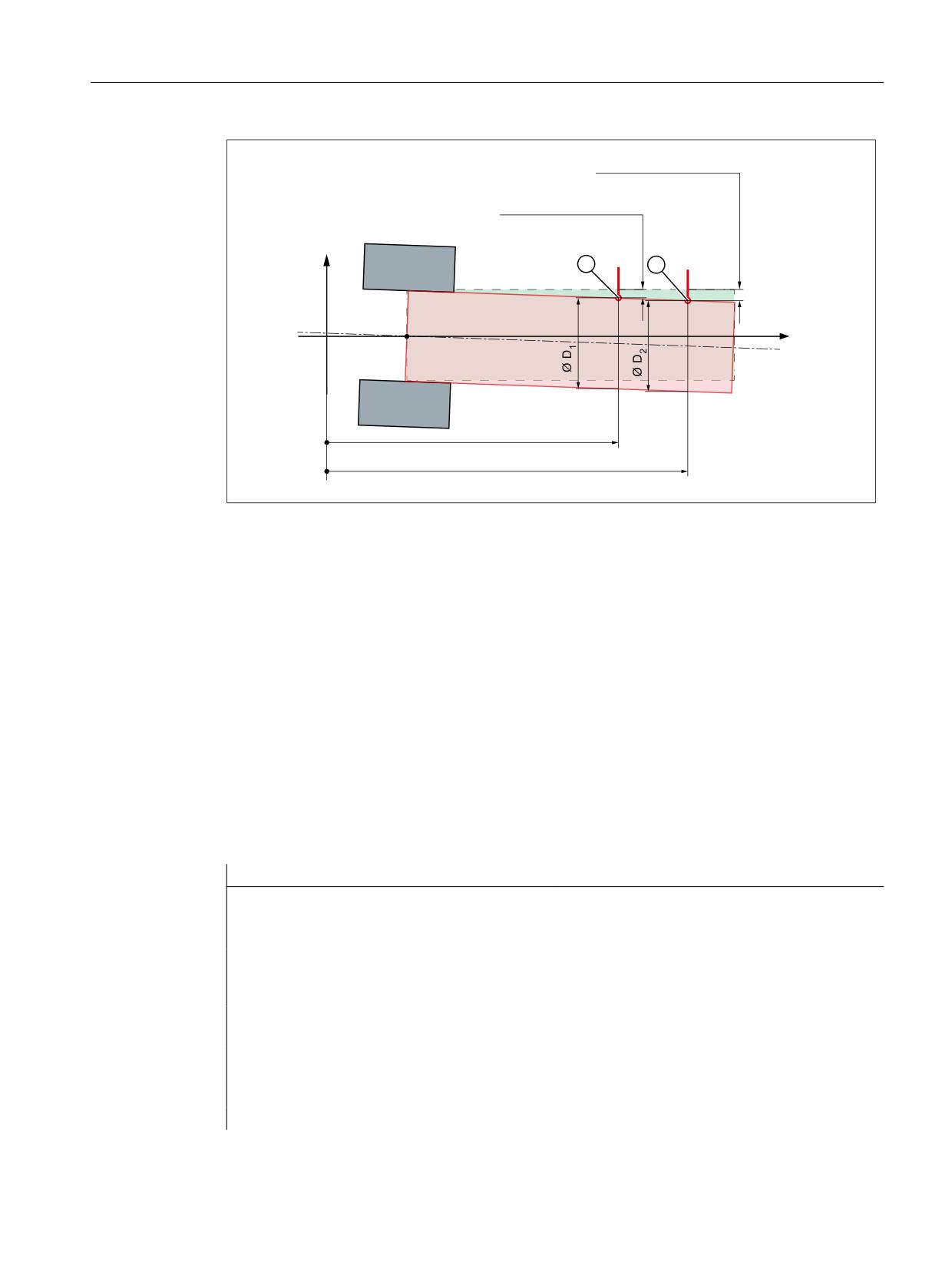
K3: Compensations
5.5 Interpolatory compensation
61B&(&B&203B > W!@
61B&(&B&203B > W!@
;
=
61B&(&B%$6B > W!@
61B&(&B%$6B > W!@
① Measuring point P1
② Measuring point P2
---
$SN_CEC_BAS_0/_1 : Positions of the measuring points in the basic axis (Z)
---
$SN_CEC_COMP_0/_1: Cylinder error at the measuring points in the compensation axis (X)
---
∅ D1 == ∅ D2
Figure 5-20
Measuring points of the cylinder error compensation
The measuring points must meet the following condition:
ZP1 < ZP2 ⇒ $SN_CEC_BAS_0 < $SN_CEC_BAS_1
Basic commissioning
Cylinder error compensation is based on sag compensation (CEC) (Page 285). As a
consequence, before commissioning the cylinder error compensation, the following
compensation parameters must first be set in the system variables of the sag compensation.
To this end, the required values are written to the system variables in an NC program.
Program code
Comment
$AN_CEC_INPUT_AXIS[<t>] = "<basic axis>"
; name of the basic axis
$AN_CEC_OUTPUT_AXIS[<t>] = "<compensa-
; name of the compensation axis
tion axis>"
$AN_CEC_MIN[<t>] = <starting position>
; starting position of the traversing
range in which the compensation should be
effective
$AN_CEC_MAX[<t>] = <end position>
; end position of the traversing range in
which the compensation should be effective
$AN_CEC_STEP[<t>] = <distance between in-
; distance between interpolation point =
terpolation points>
end position - starting position
$AN_CEC_DIRECTION[<t>] = 0
; no dependency on the direction
$AN_CEC_IS_MODULO[<t>] = FALSE
; no modulo functionality
Extended Functions
Function Manual, 12/2018, A5E40874029B AB
321

K3: Compensations
5.5 Interpolatory compensation
Program code
Comment
$AN_CEC_MULT_BY_TABLE[<t>] = 0
; no multiplication with another table
$AN_CEC_TYPE = 1
; compensation type = cylinder error com-
pensation
Distance between interpolation points ($AN_CEC_STEP[t])
Because the compensation function is a straight line, only two interpolation points are required
for the cylinder error compensation. The distance between the interpolation points is therefore
the difference between the end and the starting position:
$AN_CEC_STEP[<t>] = $AN_CEC_MAX[<t>] - $AN_CEC_MIN[<t>]
Setting the cylinder error compensation
The following shows the principle approach when setting cylinder compensation.
1. Definition of whether the actual compensation values take effect absolutely or relatively:
Setting data
Meaning
SD41356
$SN_CEC_CALC_ADD[<t>]
Absolute or additive compensation values (0: ab-
solute, 1: relative)
2. Definition of the weighting factor to which the compensation values are added:
Setting data
Meaning
SD41310
$SN_CEC_TABLE_WEIGHT[<t>]
Weighting factor
The characteristic curve can be moved vertically via the weighting factor.
3. Determining the error in the direction of the compensation axis (X) at two measuring points.
4. Transfer the measuring points (basic value and error or compensation value) to the
compensation data:
Basic value (Z)
Compensation value (X)
Measuring point
SD41330 $SN_CEC_BAS_0[<t>]
SD41340 $SN_CEC_COMP_0[<t>]
P1
Measuring point
SD41331 $SN_CEC_BAS_1[<t>]
SD41341 $SN_CEC_COMP_1[<t>]
P2
5. Triggering a positive edge change (0→1) at the start of calculation of the compensation
function:
Setting data
Meaning
SD41355
$SN_CEC_CALC[<t>]
Start of calculation by 0→1 edge
Extended Functions
322
Function Manual, 12/2018, A5E40874029B AB
K3: Compensations
5.5 Interpolatory compensation
6.
The control calculates the compensation values for the starting and end points of the
compensation straight lines, absolute or relative, depending on setting data SD41356
$SN_CEC_CALC_ADD[<t>]:
Absolute:
- SD41320 $SN_CEC_0[<t>] = <calculated compensation value at the starting position>
- SD41321 $SN_CEC_1[<t>] = <calculated compensation value at the end position>
Relative:
- SD41320 $SN_CEC_0[<t>] = SD41320 $SN_CEC_0[<t>] + <calculated compensation
value at the starting position>
- SD41321 $SN_CEC_1[<t>] = SD41321 $SN_CEC_1[<t>] + <calculated compensation
value at the end position>
Setting data
Meaning
SD41320
$SN_CEC_0[<t>]
Compensation value at the starting position
SD41321
$SN_CEC_1[<t>]
Compensation value at the end position
The measured values are written into bit memories after the calculation and then deleted:
- Bit memory = measured value
- Measured value = 0.0
Setting data
Meaning
Bit memory
SD41335
$SN_CEC_BAS_STORE_0[<t>]
Bit memories for measuring point P1: Base value
SD41350
$SN_CEC_COMP_STORE_0[<t>]
Bit memories for measuring point P1: Cylinder
error
SD41336
$SN_CEC_COMP_STORE_0[<t>]
Bit memories for measuring point P2: Base value
SD41351
$SN_CEC_COMP_STORE_1[<t>]
Bit memories for measuring point P2: Cylinder
error
Deleted measured values
SD41330
$SN_CEC_BAS_0[<t>]
Measuring point P1: Base value
SD41340
$SN_CEC_COMP_0[<t>]
Measuring point P1: Cylinder error
SD41331
$SN_CEC_BAS_1[<t>]
Measuring point P2: Base value
SD41341
$SN_CEC_COMP_1[<t>]
Measuring point P2: Cylinder error
7.
Set enable for use of the compensation table:
Setting data
Meaning
SD41300
$SN_CEC_TABLE_ENABLE[<t>]
Compensation table enable
Note
SINUMERIK Toolbox
File CNC_TAB_CONF.MPF is also provided in the SINUMERIK Toolbox. It includes an
example how cylinder error compensation can be parameterized within an NC program.
Extended Functions
Function Manual, 12/2018, A5E40874029B AB
323
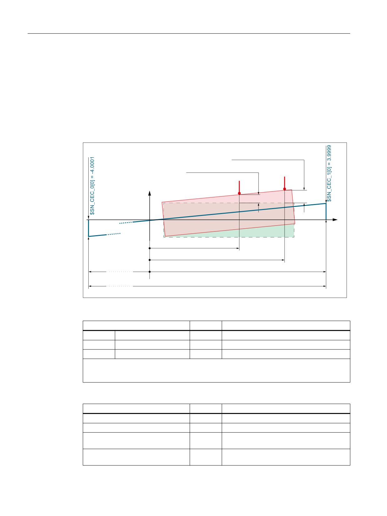
K3: Compensations
5.5 Interpolatory compensation
5.5.6.4
Examples
In the following examples, for the cylinder error compensation, the first compensation table
(index 0) is used.
Example 1: Cylinder error compensation with absolute compensation values
Overview of the compensation parameters determining the characteristic
For the example, the compensation parameters shown in the following figure are used.
61B&(&B&203B > @
61B&(&B&203B > @
;
=
61B&(&B%$6B > @
61B&(&B%$6B > @
$1B&(&B0,1> @
$1B&(&B0$;> @
$1B&(&B67(3> @
General compensation data
Setting data $SN_...
Value
Meaning
SD41300
CEC_TABLE_ENABLE[0]
FALSE
Enable
SD41310
CEC_TABLE_WEIGHT[0]
1
Weighting factor
SD41356
CEC_CALC_ADD[0]
FALSE
Absolute compensation values 1)
1) The compensation values calculated below are written into the setting data SD41320 $SN_CEC_0[0]
and SD41321 $SN_CEC_1[0], i.e. they are applied absolutely. In case of TRUE, they would be added
to the existing compensation values.
Axes, compensation range, and table properties
System variable $AN_...
Value
Meaning
CEC_INPUT_AXIS[0]
(Z)
Basic axis
CEC_OUTPUT_AXIS[0]
(X)
Compensation axis
CEC_MIN[0]
-400,000
Starting position
mm
CEC_MAX[0]
400,000
End position
mm
Extended Functions
324
Function Manual, 12/2018, A5E40874029B AB

K3: Compensations
5.5 Interpolatory compensation
System variable $AN_...
Value
Meaning
CEC_STEP[0]
800,000
Distance between interpolation points
mm
CEC_DIRECTION[0]
0
The compensation table applies to both travers-
ing directions of the basic axis.
CEC_IS_MODULO[0]
FALSE
No modulo function is active
CEC_MULT_BY_TABLE[0]
0
No table multiplication is active
Measuring points
Setting data $SN_...
Value
Meaning
SD41330
CEC_BAS_0[0]
110.0 mm
Measuring point P1: Base value
SD41331
CEC_BAS_1[0]
210.0 mm
Measuring point P2: Base value
SD41340
CEC_COMP_0[0]
0.001 mm
Measuring point P1: Cylinder error
SD41341
CEC_COMP_1[0]
0.002 mm
Measuring point P2: Cylinder error
Calculation of the compensation values
Calculation of the compensation values is performed by the control based on a rising edge
(0→1) in setting data SD41355 $SN_CEC_CALC[0]. The calculations shown below are
therefore only for illustration.
● Compensation function ΔX = f(Z):
;3
;3
˂; P
= E
= E
=3
=3
● Calculation of the gradient m:
6'
61B&(&B&203B > @
6'
61B&(&B&203B > @
P
6'
61B&(&B%$6B > @
6'
61B&(&B%$6B > @
● Calculating the offset b → measuring point P1(110.0, 0.001) and (2) used in (1):
0.001 = 1*10-5 * 110.0 + b
b = -1*10-4
(3)
● Resulting compensation function → (3) and (2) used in (1):
ΔX = 1*10-5 * Z - 1*10-4
● Calculating the compensation values → starting or end position used in (4):
SD41320 $SN_CEC_0[0] = ΔXCOMP_0 = 1*10-5 * -400000 - 1*10-4 = -4.0001
SD41321 $SN_CEC_1[0] = ΔXCOMP_1 = 1*10-5 * 400000 - 1*10-4 = 3.9999
Setting data $SN_...
Value
Meaning
SD41320
CEC_0[0]
-4.0001
Compensation value at the starting position
mm
SD41321
CEC_1[0]
3.9999
Compensation value at the end position
mm
SD41330
CEC_BAS_0[0]
0.0 mm
Measuring point P1: Base value (deleted)
SD41331
CEC_BAS_1[0]
0.0 mm
Measuring point P2: Base value (deleted)
Extended Functions
Function Manual, 12/2018, A5E40874029B AB
325

K3: Compensations
5.5 Interpolatory compensation
Setting data $SN_...
Value
Meaning
SD41335
CEC_BAS_STORE_0[0]
110.0 mm
Bit memories for measuring point P1: Base value
SD41336
CEC_BAS_STORE_1[0]
210.0 mm
Bit memories for measuring point P2: Base value
SD41340
CEC_COMP_0[0]
0.0 mm
Measuring point P1: Cylinder error (deleted)
SD41341
CEC_COMP_1[0]
0.0 mm
Measuring point P2: Cylinder error (deleted)
SD41350
CEC_COMP_STORE_0[0]
0.001 mm
Bit memories for measuring point P1: Cylinder
error
SD41351
CEC_COMP_STORE_1[0]
0.002 mm
Bit memories for measuring point P2: Cylinder
error
Example 2: Cylinder error compensation with relative compensation values
Example 2 based on the compensation data of example 1. The cylinder error compensation
is also realized using the first compensation table (index 0).
In example 2, the cylinder error is determined only at two measuring points, unlike example 1.
The compensation values are to apply relatively, i.e. they are added to the existing
compensation values from example 1.
General compensation data
Setting data $SN_...
Value
Meaning
SD41356
CEC_CALC_ADD[0]
TRUE
Relative compensation values 1)
1) The compensation values calculated below are added to the setting data SD41320 $SN_CEC_0[0]
and SD41321 $SN_CEC_1[0].
Measuring points
Setting data $SN_...
Value
Meaning
SD41330
CEC_BAS_0[0]
10.0 mm
Measuring point P1: Base value
SD41331
CEC_BAS_1[0]
410.0 mm
Measuring point P2: Base value
SD41340
CEC_COMP_0[0]
0.0 mm
Measuring point P1: Cylinder error
SD41341
CEC_COMP_1[0]
-0.003
Measuring point P2: Cylinder error
mm
Extended Functions
326
Function Manual, 12/2018, A5E40874029B AB

K3: Compensations
5.5 Interpolatory compensation
Calculation of the compensation values
Calculation of the compensation values is performed by the control based on a rising edge
(0→1) in setting data SD41355 $SN_CEC_CALC[0]:
● Compensation function: ΔX = m * Z + b = -7.5*10-6 * Z + 7.5*10-5
● Calculated compensation values:
- ΔXCOMP_0 = 3.000075 mm
- ΔXCOMP_1 = -2.999925 mm
● Adding the calculated compensation values to the actual compensation values:
- SD41320 $SN_CEC_CEC_0[0] = SD41320 $SN_CEC_CEC_0[0] + ΔXCOMP_0 = -4.0001
mm + 3.000075 = -1.000025 mm
- SD41321 $SN_CEC_CEC_1[0] = SD41321 $SN_CEC_CEC_1[0] + ΔXCOMP_1 = 3.9999
mm - 2.999925 mm = 0.999975
Setting data $SN_CEC_...
Value
Meaning
SD41320
CEC_0[0]
-1.000025
Compensation value at the starting position
mm
SD41321
CEC_1[0]
0.999975
Compensation value at the end position
mm
SD41330
CEC_BAS_0[0]
0.0 mm
Measuring point P1: Base value (deleted)
SD41331
CEC_BAS_1[0]
0.0 mm
Measuring point P2: Base value (deleted)
SD41335
CEC_BAS_STORE_0[0]
10.0 mm
Bit memories for measuring point P1: Base value
SD41336
CEC_BAS_STORE_1[0]
410.0 mm
Bit memories for measuring point P2: Base value
SD41340
CEC_COMP_0[0]
0.0 mm
Measuring point P1: Cylinder error (deleted)
SD41341
CEC_COMP_1[0]
0.0 mm
Measuring point P2: Cylinder error (deleted)
SD41350
CEC_COMP_STORE_0[0]
0.0 mm
Bit memories for measuring point P1: Cylinder
error
SD41351
CEC_COMP_STORE_1[0]
-0.003
Bit memories for measuring point P2: Cylinder
mm
error
5.5.7
Supplementary conditions
Compensated actual position
The following functions are based on the compensated actual position:
● Measurement
● Teach In
● Software limit switch
Extended Functions
Function Manual, 12/2018, A5E40874029B AB
327
K3: Compensations
5.5 Interpolatory compensation
Displaying the actual position
The actual position of the axis without compensation (ideal machine) is displayed in the actual
position display in the machine coordinate system.
The actual position of the axis with compensation (MSEC and backlash compensation) is
displayed in the service display "Axis/spindle" ("Diagnostics" operating area).
Displaying the compensation values
The following compensation values are also output in the "Axis/spindle" service display
(operating area "Diagnosis"):
● "Absolute compensation value measuring system 1" or 2
The value displayed is the sum of the compensation values of MSEC, obtained from the
actual position of the basic and compensation axis, and backlash compensation.
● Compensation, sag + temperature
The value displayed is the sum of the compensation values of sag and temperature
compensation, obtained from the actual position of the basic and compensation axis.
Loss of the referenced status of the basic axis
If the referenced status of the active measuring system of the basic axis changes from
"Referenced/synchronized" to "Not referenced/synchronized" (DB31, ... DBX60.4 or .5: 1→0),
then the MSEC and/or sag compensation is deactivated in the corresponding axis (basic/
compensation axis).
If the referenced status of the active measuring system of the basic axis then changes from
"Not referenced/synchronized" to "Referenced/synchronized" (DB31, ... DBX60.4 or .5: 0→1),
then the MSEC and/or sag compensation is reactivated in the corresponding axis (basic/
compensation axis).
Controller enable signals
If a compensation relationship is active, then the controller enable (DB31, ... DBX2.1) should
always be set the same for the basic and compensation axes.
Traversing signal output
The traversing signals of the compensation axis are only when the compensation function is
activated/deactivated and when the number of active compensation tables changes.
Traversing motion of the compensation axis, resulting from motion of the basic axis, does not
result in the output of traversing signals in the compensation axis.
Extended Functions
328
Function Manual, 12/2018, A5E40874029B AB

K3: Compensations
5.6 Dynamic feedforward control (following error compensation)
5.6
Dynamic feedforward control (following error compensation)
5.6.1
General properties
Axial following error
The remaining system deviation of the position controller when traversing a machining axis is
known as axial following error. Expressed in another way, the axial following error is the
difference between the setpoint position and the actual position of the machine axis.
Effects
Particularly during acceleration in contour curvatures, e.g. circles and corners, this following
error leads to undesirable, velocity-dependent contour violations.
Compensation
The axial following error can be reduced almost to zero with the help of the "dynamic
feedforward control". The function is therefore also called "following error compensation".
Methods
There are two "dynamic feedforward control" methods:
● Speed feedforward control (velocity-dependent)
● Torque feedforward control (acceleration-dependent)
Activation
The feedforward control method is selected and activated using the machine data:
MD32620 $MA_FFW_MODE (feedforward control mode)
Value
Meaning
0
No feedforward control
1
Speed feedforward control with PT1 balancing
2
Torque feedforward control with PT1 balancing
3
Speed feedforward control with Tt balancing
4
Torque feedforward control with Tt balancing
Activation/deactivation in part program
The following axis-specific machine data can be used to define that the feedforward control
for the respective axis/spindle can be activated and deactivated by the part program:
Extended Functions
Function Manual, 12/2018, A5E40874029B AB
329

K3: Compensations
5.6 Dynamic feedforward control (following error compensation)
MD32630 $MA_FFW_ACTIVATION_MODE (activate feedforward control from program)
Value
Meaning
0
The feedforward control cannot be activated and deactivated from the part program. This
means that the state specified using MD32620 $MA_FFW_MODE is always effective for the
axis/spindle.
1
The feedforward control can be activated and deactivated from the part program. The operation
becomes active immediately.
2
The feedforward control can be activated and deactivated from the part program. The operation
only becomes active the next time that the axis comes to a standstill.
The feedforward control is activated/deactivated from the part program using the operations:
FFWON: Feedforward control ON
FFWOF: Feedforward control OFF
The default setting (i.e. M30 even after reset) is entered using the channel-specific machine
data:
MD20150 $MC_GCODE_RESET_VALUES (initial setting of the G groups)
FFWON/FFWOF is active for all axes/spindles in the axis mode, where:
MD32630 $MA_FFW_ACTIVATION_MODE = 1 (or 2)
and
MD32620 $MA_FFW_MODE = 1, 2, 3 or 4
The identical MD32630 setting should be used for axes that interpolate with each other.
The feedforward control should only be activated or deactivated while the axis/spindle is
stationary in the axis mode, in order to prevent jerky motion. Hence the switchover is delayed
automatically up to the next standstill through block search stop.
Note
A preprocessing stop has no effect for command or PLC axes traversing asynchronously to
the part program processing. To ensure that FFWON/FFWOF only has an effect on the axis/
spindle when it is next stationary in the axis mode, you must explicitly set MD32630 = 2 for
each axis/spindle in the axis mode (see also "Forward feed control for command- and PLC
axes (Page 335)").
5.6.2
Speed feedforward control
Function
In the case of speed feedforward control, a velocity setpoint is also applied directly to the input
of the speed controller. With this value the following error can be reduced to nearly zero (i.e.
system deviation is 0) when the velocity is constant.
Extended Functions
330
Function Manual, 12/2018, A5E40874029B AB
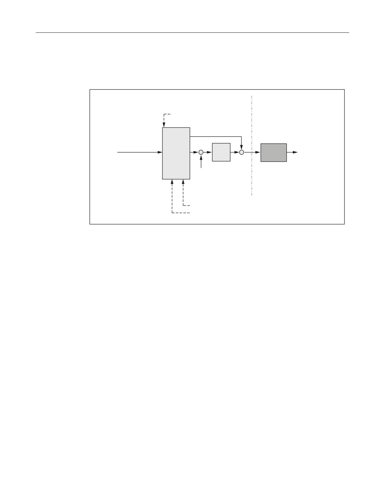
K3: Compensations
5.6 Dynamic feedforward control (following error compensation)
Commissioning
The following axis-specific parameters must be defined for the speed feedforward control
during commissioning:
1&.
'ULYH
0'
0$B )):B02'(
3RVLWLRQ
6HWSRLQW
)HHGIRUZDUG
6SHHG
FRQ
UHIHUHQFH YDOXH
FRQWURO
FRQWUROOHU
WUROOHU
3RVLWLRQ DFWXDO YDOXH
0'
0$B9(/2B)):B:(,*+7
0'
0$B(48,9B63(('&75/B7,0(
Equivalent time constant of the speed control loop (MD32810)
The equivalent time constant of the speed control loop must be determined accurately (e.g.
graphically from a speed setpoint step response) and entered into the following machine data
to correctly set the speed feedforward control:
MD32810 $MA_EQUIV_SPEEDCTRL_TIME (equivalent time constant speed control loop for
feedforward control)
Feedforward control factor for speed feedforward control (MD32610)
The additional velocity setpoint can be weighted using a factor:
MD32610 $MA_VELO_FFW_WEIGHT
Range of values: 0 ... 1
"0" means: no feedforward control. As standard, the factor has a value of 1 (≙ 100%).
The factor should remain set at 100%, as this value is the optimum setting for an optimally set
control loop for the axis/spindle as well as a precisely determined equivalent time constant of
the speed control loop.
Fine adjustment
The speed feedforward control for the particular axis/spindle can be optimized by making slight
changes (fine tuning) to the equivalent time constants of the speed control loop (MD32810).
To make this check, the axis/spindle should be traversed at a constant velocity and in the
service display "Axis/spindle", the "System deviation" should be checked.
A small acceleration and a high feedrate should be chosen so that the values can be easily
read on the service display. This produces very long acceleration phases from which it is easy
to read off the control deviation.
Extended Functions
Function Manual, 12/2018, A5E40874029B AB
331
K3: Compensations
5.6 Dynamic feedforward control (following error compensation)
Example:
MD32300 $MA_MAX_AX_ACCEL = 0.1
; Maximum axis acceleration = 0.1 m/s2
MD32000 $MA_MAX_AX_VELO = 20000.0
; Maximum axis velocity
= 20000.0 mm/min
; Part program for setting the equivalent time constant
G1 F20000
FFWON
LOOP:
X1000
X0
GOTOB LOOP
M30
References
For detailed information about setting the equivalent time constants of the speed control loop
(MD32810) refer to:
● Function Manual, Basic Functions; Velocities, Setpoint / Actual Value Systems, Closed-
Loop Control (G2), Section: Optimization of the control
5.6.3
Torque feedforward control
Function
In the case of torque feedforward control, an additional current setpoint proportional to the
torque is applied directly to the current controller input. This value is formed using the
acceleration and moment of inertia.
Application
Torque feedforward control is required to achieve high contour accuracy where the demands
on the dynamic response are very high. If set correctly, the following error can almost be
completely compensated even during high acceleration.
Extended Functions
332
Function Manual, 12/2018, A5E40874029B AB
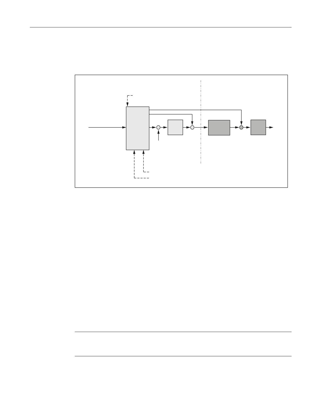
K3: Compensations
5.6 Dynamic feedforward control (following error compensation)
Commissioning
The following axis-specific parameters must be defined during commissioning for torque
feedforward control:
1&.
'ULYH
0'
0$B )):B02'(
3RVLWLRQ
&XUUHQW
6HWSRLQW
3UHFRQ
6SHHG
FRQWURO
FRQWURO
VHWSRLQW
WURO
FRQWUROOHU
OHU
OHU
$FWXDO SRVLWLRQ
YDOXH
0'
0$B$;B,1(57,$
0'
0$B(48,9B&855&75/B7,0(
Equivalent time constant of the current control loop (MD32800)
The equivalent time constant of the current control loop must be determined accurately (e.g.
graphically from the step response of the current control loop) and entered in the following
machine data in order to correctly set the torque feedforward control:
MD32800 $MA_EQUIV_CURRCTRL_TIME (equivalent time constant current control loop for
feedforward control)
Total moment of inertia of axis (MD32650)
The total moment of inertia (moment of inertia of drive plus load referred to the motor shaft) of
the axis must be determined and entered in the following machine data:
MD32650 $MA_AX_INERTIA (inertia for torque feedforward control)
Fine adjustment
The torque feedforward control for the particular axis/spindle can be optimized by making slight
changes (fine tuning) to the values in MD32800 and MD32650.
To make a check, the following error should be recorded via the trace functionality. In addition
to traversing at a constant velocity, the following error should be monitored especially when
the axis/spindle accelerates.
Note
As a result of the extremely fast sequences when accelerating, when commissioning the torque
feedforward control, the service display cannot be used to check the fine adjustment.
Extended Functions
Function Manual, 12/2018, A5E40874029B AB
333
K3: Compensations
5.6 Dynamic feedforward control (following error compensation)
References
For detailed information about setting the equivalent time constants of the current control loop
(MD32810) refer to:
● Function Manual, Basic Functions; Velocities, Setpoint / Actual Value Systems, Closed-
Loop Control (G2), Section: Optimization of the control
5.6.4
Dynamic response adaptation
Function
For axes that interpolate with one another, but with different axial control loop response times,
dynamic response adaptation can be used to achieve identical time responses of all axes to
ensure optimum contour accuracy without loss of control quality.
Commissioning
Time constant for dynamic response adaptation (MD32910)
The difference between the equivalent time constants of the "slowest" speed or current control
loop and the particular axis should be entered as time constant for the dynamic response
adaptation in the following machine data.
MD32910 $MA_DYN_MATCH_TIME (time constant of dynamic response adaptation)
Example:
Equivalent time constants of the speed control loop (MD32810) for active speed feedforward
control of axes 1, 2 and 3:
● Axis 1: 2 ms
● Axis 2: 4 ms (dynamically the slowest axis)
● Axis 3: 1 ms
This means that the following values are obtained for the time constant of the dynamic
response adaptation MD32910:
● Axis 1: 2 ms
● Axis 2: 0 ms
● Axis 3: 3 ms
Activation (MD32900)
The dynamic response adaptation is only active if the following machine data is set:
MD32900 $MA_DYN_MATCH_ENABLE= 1
References
Function Manual, Basic Functions; Velocities, Setpoint-Actual Value Systems, Closed-Loop
Control (G2), Chapter: "Optimizing the closed-loop control"
Extended Functions
334
Function Manual, 12/2018, A5E40874029B AB
K3: Compensations
5.6 Dynamic feedforward control (following error compensation)
5.6.5
Forward feed control for command- and PLC axes
Function
For command and PLC axes, it must be prevented that the feedforward control is activated/
deactivated at higher velocities as follows:
MD32630 $MA_FFW_ACTIVATION_MODE = 2
With this setting, the FFWON/FFWOF operation only becomes active below the stationary
velocity (MD36060 $MA_STANDSTILL_VELO_TOL) configured for this particular axis.
If the switchover instruction coincides with an axis motion, the required switchover is executed
only in the next stoppage condition of the axis. This avoids the following error being suddenly
established/reduced.
Note
A stoppage velocity set to a very high value can lead to the changeover of the feedforward
control in the movement. Controls can be activated depending on the existing following error.
Commissioning
We recommend the following procedure when checking the feedforward control for command
and PLC axes:
1. Check the stoppage velocity in MD36060.
2. Check the existing following error of the axis in stoppage condition.
3. Setting the changeover condition and activating it:
MD32630 = 2
4. Traverse axis in the part program using the POSA operation.
5. Execute FFWON during the axis motion.
6. The KV factor and following error displayed in the service display "Axis/spindle" must not
jump.
7. A higher KV factor and a lower following error are only obtained for traversing motion
following standstill. However, the feedforward control is active only from the stoppage
condition.
Essentially the same as when activating the feedforward control, for deactivation, the following
applies:
1. Traverse axis in the part program using the POSA operation.
2. Execute FFWOF during the axis motion.
3. The KV factor and following error displayed in the service display "Axis/spindle" must not
jump.
4. A lower KV factor and a higher following error are only obtained for traversing motion
following standstill. However, the feedforward control is inactive only from the stoppage
condition.
Extended Functions
Function Manual, 12/2018, A5E40874029B AB
335
K3: Compensations
5.6 Dynamic feedforward control (following error compensation)
Example
In the following program example, axis A is traversed asynchronously to the path. An attempt
is made to activate the feedforward control in the channel while traversing. Contrary to the
geometry axes X, Y and Z, the feedforward control is not immediately effective for axis A. Here
one waits for the stoppage after N60. Axis A then traverses with the feedforward control in
N70.
Program code
N10 FFWOF
N20 POSA[A]=1000 FA[A]=10000
N30 G4 F1
N40 FFWON
N50 G0 X10 Y10 Z10
N60 WAITP(A)
N70 POSA[A]=1500 FA[A]=10000
N80 WAITP(A)
M30
5.6.6
Secondary conditions
Axes that are interpolating axes with one another
Also for axes that interpolate with one another, the feedforward control parameter should be
optimally set for each axis, i.e. also several axes that are interpolating with one another can
have different feedforward control parameters.
Check contour monitoring
As the two equivalent time constants:
● MD32810 $MA_EQUIV_SPEEDCTRL_TIME (equivalent time constant speed control loop
for feedforward control)
and
● MD32800 $MA_EQUIV_CURRCTRL_TIME) (equivalent time constant current control loop
for feedforward control)
also influence the contour monitoring, this should be subsequently checked.
References:
Function Manual, Basic Functions; Axis Monitoring, Protection Zones (A3)
Extended Functions
336
Function Manual, 12/2018, A5E40874029B AB
K3: Compensations
5.7 Friction compensation overview
Influence on the servo gain factor (K
factor)
V
When the feedforward control is set correctly, the response to setpoint changes in the
controlled system under speed feedforward control is as dynamic as that of the speed control
loop or, under torque feedforward control, as that of the current control loop, i.e. the servo gain
factor (KVfactor) entered into MD32200 $MA_POS_CTRLGAIN hardly has any effect on the
control behavior (e.g. corner errors, overshoots, circle/radius errors).
On the other hand, feedforward control does not affect the response to disturbances
(synchronism). In this case, the servo gain factor (KV factor) entered in MD32200 is the active
factor.
Service display "KV factor"
When a feedforward control is active, the servo gain (KV factor) of the axis (corresponds to
servo gain factor (KVfactor) active as response to setpoint changes) shown in the service
display "axis/spindle" is very high.
5.7
Friction compensation overview
In addition to the mass inertia and the machining forces, the friction forces in the gearing and
guideways of the machine influence the dynamic behavior of a machine axis. In particular,
when accelerating a machine axis from standstill, the transition from static to sliding friction
has an adverse effect. The resulting sudden change in the friction force results in a briefly
increased following error. With interpolating axes, this results in significant contour violations.
For circles, these occur especially at the quadrant transitions where one of the participating
axes is stationary as its direction is reversed.
To improve the contour accuracy at these points, an additional setpoint pulse (velocity or torque
setpoint pulse) is applied to the friction compensation when a machine axis is accelerated from
standstill.
Extended Functions
Function Manual, 12/2018, A5E40874029B AB
337
K3: Compensations
5.8 Friction compensation with a constant compensation value
Friction compensation functions
The following functions are available for friction compensation:
● Friction compensation with a constant compensation value (Page 338)
Depending on the acceleration of the machine axis, the same pulse is always applied to
the velocity setpoint.
The amplitude and the decay time of the velocity setpoint pulse can be set.
● Friction compensation with adaptive characteristic (Page 344)
Depending on the acceleration of the machine axis, the velocity setpoint pulse is determined
from a parameterizable characteristic.
Three different acceleration values can be set as well as the minimum and maximum
amplitude and the decay time of the velocity setpoint pulse.
● Friction compensation with adaptive characteristics (Page 347) (Licensed option:
6FC5800-0AS06-0YB0)
Depending on the acceleration of the machine axis, the velocity setpoint pulse is determined
from up to three parameterizable characteristics.
Up to nine different acceleration values can be set. For each acceleration value, weighting
factors for the amplitude, the active time, and the decay time of the velocity setpoint pulse
can be defined.
If the velocity setpoint pulse is not sufficient to achieve the desired result, an additional
torque setpoint pulse can be parameterized.
5.8
Friction compensation with a constant compensation value
5.8.1
Description of functions
The friction compensation described below with constant compensation value is intended for
applications in which the following general conditions apply:
● The velocity setpoint pulse required for friction compensation is independent of the
acceleration.
● An acceleration-independent amplitude and an acceleration-independent decay time are
sufficient to model the velocity setpoint pulse.
● For friction compensation at the positive and negative reversal point, the same velocity
setpoint pulse is sufficient.
● The requirement for contour accuracy at the reversal points is relatively low.
The following figure shows an example characteristic that can be set with this function:
Extended Functions
338
Function Manual, 12/2018, A5E40874029B AB
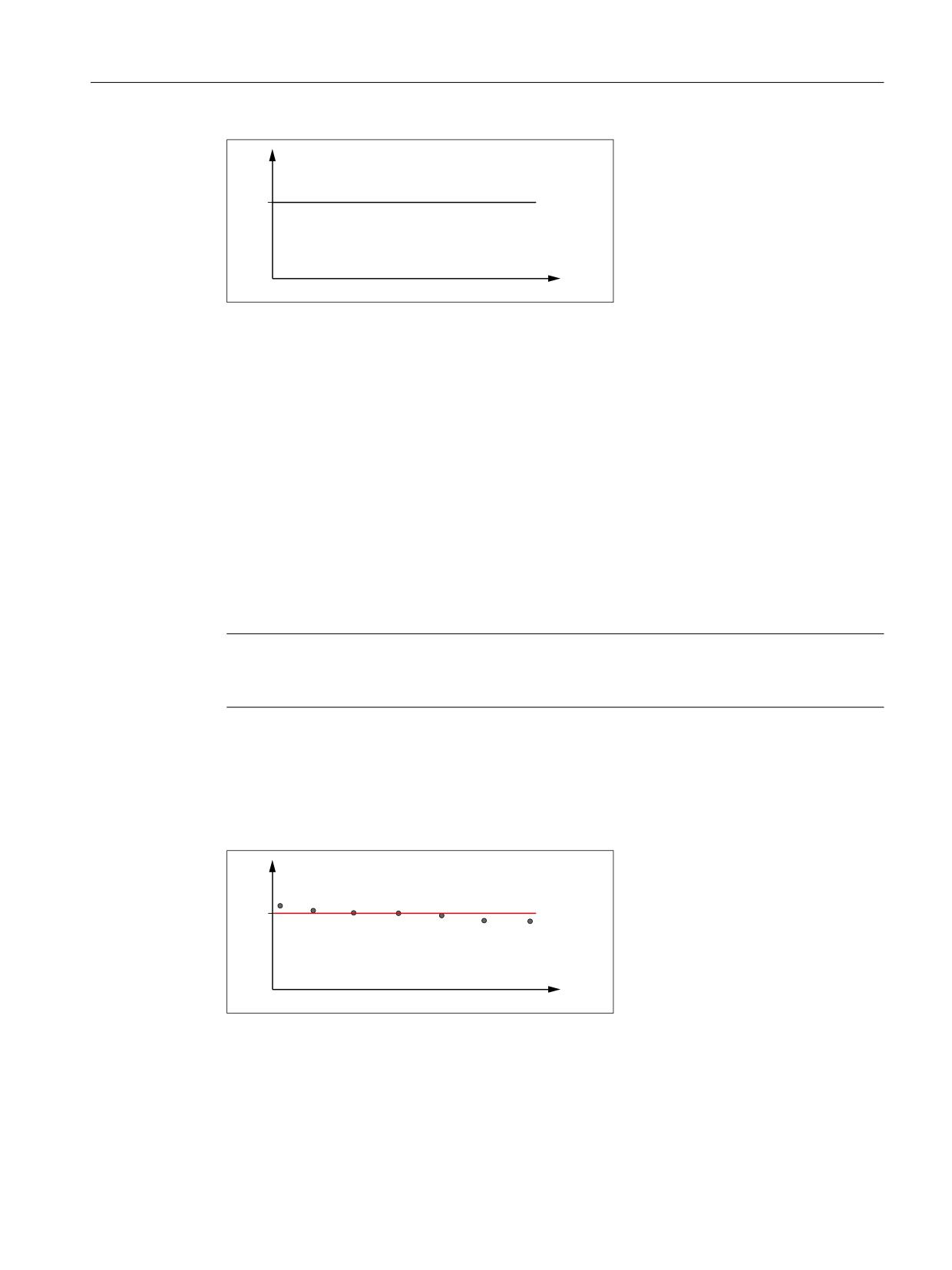
K3: Compensations
5.8 Friction compensation with a constant compensation value
˂Q
˂QRSW
D
Δnopt
Amplitude of the velocity setpoint pulse
a
Acceleration at the quadrant transition
5.8.2
Commissioning
To determine the axis-specific compensation value Δnopt, the Circularity test (Page 340) must
be used to determine the optimum amplitude of the velocity setpoint pulse Δnopt_a for each of
a number of acceleration values. The different acceleration values should cover the entire
dynamic range.
Calculation of the acceleration at the quadrant transition
On a circular path, the acceleration a of a machine axis on direction reversal at the quadrant
transition is calculated from the radius r of the circle and the path velocity v: a = v2 / r
Note
The path velocity and therefore the axis-specific acceleration a can be varied simply via the
feedrate override.
Evaluation of the value pairs determined (a, Δnopt_a)
To determine the compensation value Δnopt, we recommend graphically applying the value
pairs determined in the circularity test comprising the acceleration a and the associated
optimum amplitude of the velocity setpoint pulse Δnopt_a: Δnopt_a = f(a)
˂Q
˂QRSW
*
D
Figure 5-21
Axis-specific characteristic determination
The optimum amplitude of the velocity setpoint pulse Δnopt is obtained by drawing in the straight
line G1.
Extended Functions
Function Manual, 12/2018, A5E40874029B AB
339
K3: Compensations
5.8 Friction compensation with a constant compensation value
Axis-specific machine data
Activating friction compensation
Friction compensation is activated with:
● MD32500 $MA_FRICT_COMP_ENABLE[ <axis> ] = TRUE (1)
Activating friction compensation with a constant compensation value
Friction compensation with constant compensation value is activated with:
● MD32490 $MA_FRICT_COMP_MODE[ <axis> ] = 1
● MD32510 $MA_FRICT_COMP_ADAPT_ENABLE[ <axis> ] = FALSE (0)
Velocity setpoint pulse: Amplitude
The amplitude of the velocity setpoint pulse is set with:
MD32520 $MA_FRICT_COMP_CONST_MAX[ <axis> ] = <amplitude>
Velocity setpoint pulse: Decay time
The decay time of the velocity setpoint pulse is set via:
MD32540 $MA_FRICT_COMP_TIME[ <axis> ] = <time constant>
5.8.2.1
Circularity test
Commissioning via the circularity test
The easiest way to commission the friction compensation is with the circularity test integrated
in the user interface. This involves acquiring the circular contour created on the machine as a
circle is traversed based on the actual positions of the participating machine axes. Deviations
from the programmed ideal circular contour, in particular, at the quadrant transitions, are
visualized graphically.
The circularity test can be found on the user interface under:
● SINUMERIK Operate: "Operating area switchover" > "Commissioning" > "Optimization/
test" > "Circularity test"
Sequence
The sequence for commissioning friction compensation for a machine axis is divided into the
following steps:
1. Set the acceleration a1 via path velocity vn and circle radius r
2. Perform circularity test without friction compensation
3. Perform a circularity test with friction compensation with small initial values for amplitude
and decay time
4. Optimize the circularity test with friction compensation by changing the parameter values
step by step
Extended Functions
340
Function Manual, 12/2018, A5E40874029B AB
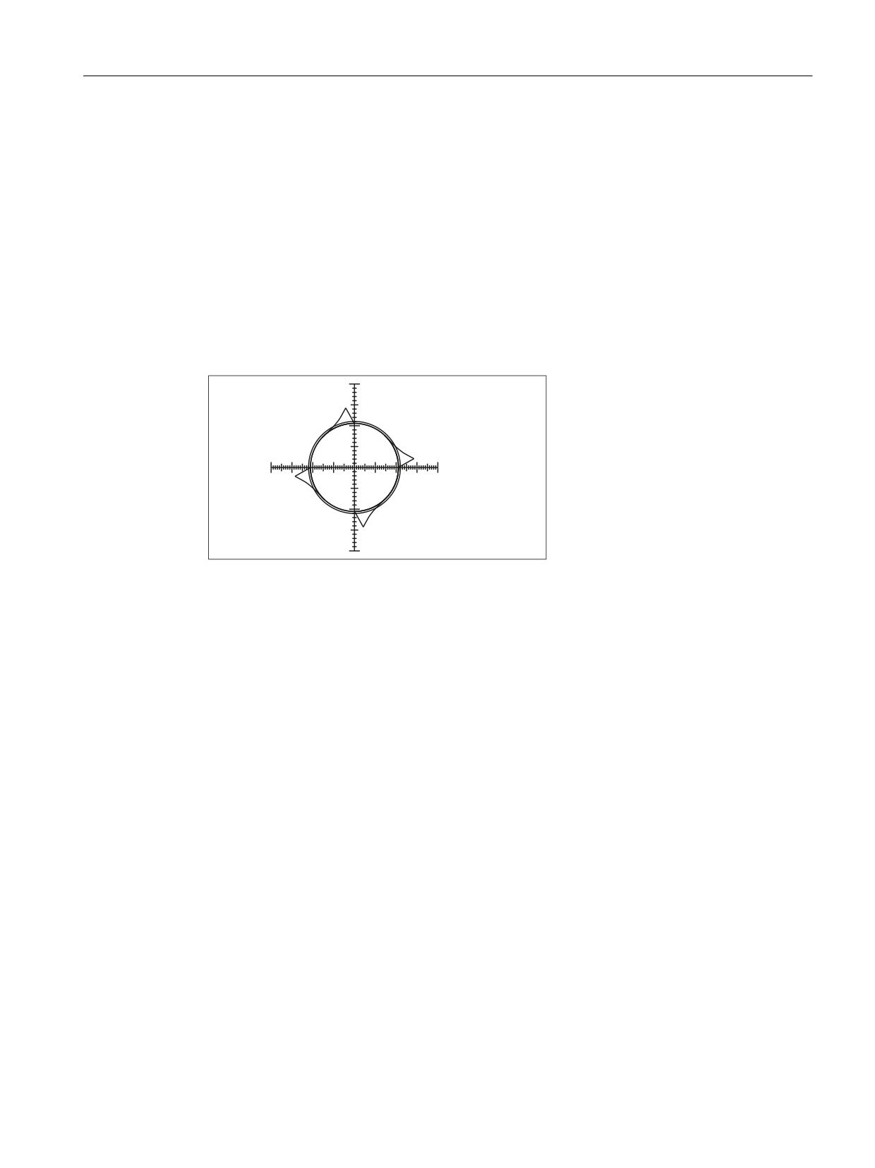
K3: Compensations
5.8 Friction compensation with a constant compensation value
5. The optimized parameter values are applied graphically, e.g. amplitude = f(a
n
)
6. Setting of the next acceleration an and continuation with point 2.
Performing the circularity test without friction compensation
A circularity test without friction compensation should be performed to determine the initial
quality of the circular contour at the quadrant transitions. To do this, switch off the friction
compensation temporarily:
MD32500 FRICT_COMP_ENABLE[ <axis> ] = 0
The following figure shows a typical example of quadrant transitions without friction
compensation:
$[LV
,,
,
$[LV
,,,
,9
Figure 5-22
Quadrant transitions without friction compensation
The friction compensation must then be activated again:
MD32500 FRICT_COMP_ENABLE[ <axis> ] = 1
Performing circularity test with friction compensation
It is recommended that a small amplitude value and a decay time of just a few position control
cycles be set as initial values for the velocity setpoint pulse, e.g.:
● MD32520 $MA_FRICT_COMP_CONST_MAX[ <axis> ] = 10 [mm/min]
● MD32540 $FRICT_COMP_TIME[ <axis> ] = 0.008 [s]
The circularity test performed with these values provides an initial assessment of the friction
compensation.
Amplitude too small
Too small an amplitude value (MD32520) is revealed in the circularity test by insufficient
compensation of the contour deviations at the quadrant transitions.
Extended Functions
Function Manual, 12/2018, A5E40874029B AB
341
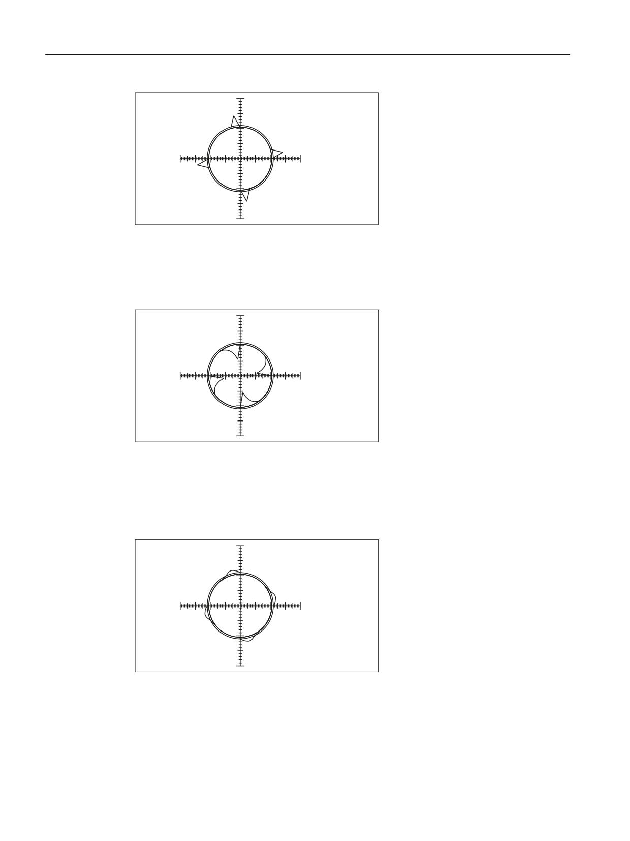
K3: Compensations
5.8 Friction compensation with a constant compensation value
$[LV
,,
,
$[LV
,,,
,9
Figure 5-23
Amplitude too small
Amplitude too large
Too large an amplitude value (MD32520) is revealed in the circularity test by overcompensation
of the contour deviations at the quadrant transitions.
$[LV
,,
,
$[LV
,,,
,9
Figure 5-24
Amplitude too large
Decay time too short
Too short a decay time (MD32540) is revealed in the circularity test when the contour deviations
at the quadrant transitions are compensated for for a short time but immediately increase again
thereafter.
$[LV
,,
,
$[LV
,,,
,9
Figure 5-25
Decay time too short
Decay time too long
Too long a decay time (MD32540) is revealed in the circularity test when the contour deviation
at the quadrant transitions is compensated for at first. This assumes that the optimum
Extended Functions
342
Function Manual, 12/2018, A5E40874029B AB
K3: Compensations
5.8 Friction compensation with a constant compensation value
amplitude values has already been set. If the decay time is too long, however, the
compensation applies for too long and results in overcompensation at the next circular contour.
$[LV
,,
,
$[LV
,,,
,9
Figure 5-26
Decay time too long
Good friction compensation setting
With a good friction compensation setting, "no" contour violations can be detected at the
quadrant transitions.
$[LV
,,
,
$[LV
,,,
,9
Figure 5-27
Good friction compensation setting
See also
Friction compensation with adaptive characteristic (Page 344)
5.8.3
Supplementary conditions
Reaction of setpoint-related compensation functions
The following setpoint-related compensation functions affect the position setpoint and must
therefore be deactivated for the axes that perform a circularity test:
● Sag and angularity compensation (CEC)
MD32710 $MA_CEC_ENABLE[ <axis> ] = 0
● Directional leadscrew error compensation (LEC):
MD32710 $MA_CEC_ENABLE[ <axis> ] = 0
● Temperature compensation:
MD32750 $MA_TEMP_COMP_TYPE[ <axis> ] = 0
Extended Functions
Function Manual, 12/2018, A5E40874029B AB
343
K3: Compensations
5.9 Friction compensation with adaptive characteristic
5.9
Friction compensation with adaptive characteristic
5.9.1
Description of functions
The friction compensation with adaptive characteristic is intended for applications with the
following requirements:
● The velocity setpoint pulse required for friction compensation depends on the acceleration.
● It is enough if the characteristic is modeled by three different acceleration interpolation
points and a minimum and maximum amplitude of the velocity setpoint pulse.
● An acceleration-dependent amplitude and an acceleration-independent decay time are
sufficient to model the velocity setpoint pulse.
● For friction compensation at the positive and negative reversal point, the same velocity
setpoint pulse is sufficient.
● For greater acceleration, a smaller compensation value is required than for smaller
acceleration.
● The requirement for contour accuracy at the reversal points is high.
The following figure shows an example characteristic that can be set with this function:
˂Q
˂QPD[
˂QPLQ
D
D
D
D
%
%
%
%
Δnmax
Maximum amplitude of the velocity setpoint pulse
Δnmin
Minimum amplitude of the velocity setpoint pulse
a1, a2,
Acceleration interpolation points 1, 2, and 3
a3
B1 ... Acceleration range 1 ... 4
B4
Extended Functions
344
Function Manual, 12/2018, A5E40874029B AB
K3: Compensations
5.9 Friction compensation with adaptive characteristic
The amplitude of the velocity setpoint pulse Δn is calculated in the relevant acceleration range
B1 to B4 to form:
Range
Acceleration a
Amplitude of the velocity setpoint pulse Δn
B1
a < a1
Δn = Δnmax * a / a1
B2
a1 ≤ a ≤ a2
Δn = Δnmax
B3
a2 < a < a3
Δn = Δnmax + [(Δnmin - Δnmax) / (a3 - a2)] * (a - a2)
B4
a ≥ a3
Δn = Δnmin
5.9.2
commissioning
To determine the axis-specific characteristic parameters, the Circularity test (Page 340) must
be used to determine the optimum amplitude of the velocity setpoint pulse Δnopt_a each for each
of a number of acceleration values. The different acceleration values should cover the entire
dynamic range. In particular, a sufficient number of measurements must be ensured for low
acceleration values and large circle radii.
Calculation of the acceleration at the quadrant transition
On a circular path, the acceleration a of a machine axis on direction reversal at the quadrant
transition is calculated from the radius r of the circle and the path velocity v: a = v2 / r
Note
The path velocity and therefore the axis-specific acceleration a can be varied simply via the
feedrate override.
Evaluation of the value pairs determined (a, Δnopt_a)
To determine the acceleration interpolation points a1, a2, and a3 and the minimum and
maximum amplitude of the velocity setpoint pulse Δnmin and Δnmax, we recommend graphically
applying the value pairs determined in the circularity test comprising the acceleration a and
the associated optimum amplitude of the velocity setpoint pulse Δnopt_a: Δnopt_a = f(a)
˂Q
*
*
˂QPD[
*
˂QPLQ
*
D
D
D
D
%
%
%
%
Figure 5-28
Axis-specific characteristic determination
Extended Functions
Function Manual, 12/2018, A5E40874029B AB
345
K3: Compensations
5.9 Friction compensation with adaptive characteristic
The acceleration interpolation points a
1
, a2, and a3 and the minimum and maximum amplitude
of the velocity setpoint pulse Δnmin and Δnmax result from drawing in the straight lines G1 ...G4.
Axis-specific machine data
Activating friction compensation
Friction compensation is activated with:
MD32500 $MA_FRICT_COMP_ENABLE[ <axis> ] = TRUE (1)
Activating friction compensation with adaptive characteristic
Friction compensation with adaptive characteristic is activated with:
● MD32490 $MA_FRICT_COMP_MODE[ <axis> ] = 1
● MD32510 $MA_FRICT_COMP_ADAPT_ENABLE[ <axis> ] = TRUE (1)
Characteristic parameters: Acceleration a1, a2, and a3
The axis-specific acceleration a occurring on a circle path on reversal at the quadrant
transitions is calculated from the radius r and the path velocity v as: a = v2 / r
The acceleration values a1, a2, and a3, are entered in the machine data in monotonically
ascending order (a1 < a2 < a3).
● MD32550 $MA_FRICT_COMP_ACCEL1[ <axis> ] = <a1>
● MD32560 $MA_FRICT_COMP_ACCEL2[ <axis> ] = <a2>
● MD32570 $MA_FRICT_COMP_ACCEL3[ <axis> ] = <a3>
Characteristic parameters: Amplitude Δnmin and Δnmax
The maximum and minimum amplitude of the velocity setpoint pulse (Δnmax, Δnmin) must be
entered in the following machine data:
● MD32520 $MA_FRICT_COMP_CONST_MAX[ <axis> ] = <Δnmax>
● MD32530 $MA_FRICT_COMP_CONST_MIN[ <axis> ] = <Δnmin>
Note
If satisfactory results cannot be obtained for very small path velocities, the computational
resolution may have to be increased:
● MD10200 $MA_INT_INCR_ PER_MM (computational resolution for linear positions)
● MD10210 $MA_INT_INCR_PER_DEG (computational resolution for angular positions)
Velocity setpoint pulse: Decay time
The decay time of the velocity setpoint pulse is set via:
MD32540 $MA_FRICT_COMP_TIME[ <axis> ] = <decay time>
Extended Functions
346
Function Manual, 12/2018, A5E40874029B AB
K3: Compensations
5.10 Friction compensation with adaptive characteristics
5.9.3
Supplementary conditions
Reaction of setpoint-related compensation functions
The following setpoint-related compensation functions affect the position setpoint and must
therefore be deactivated for the axes that perform a circularity test:
● Sag and angularity compensation (CEC)
MD32710 $MA_CEC_ENABLE[ <axis> ] = 0
● Directional leadscrew error compensation (LEC):
MD32710 $MA_CEC_ENABLE[ <axis> ] = 0
● Temperature compensation:
MD32750 $MA_TEMP_COMP_TYPE[ <axis> ] = 0
5.10
Friction compensation with adaptive characteristics
5.10.1
Description of the function
Friction compensation with adaptive characteristics has the following properties:
● For fast and simple optimization, commissioning can be performed via the SINUMERIK
Operate user interface.
● In guided commissioning, the test movements are optionally generated automatically for
one or two axes.
● The compensation values can be set separately for each axis, e.g. for a vertical axis, for
each reversal point.
● In relation to the set position (compensation mode (Page 349) = 3), better results are
achieved by early application of the compensation value.
● If the velocity setpoint pulse is insufficient to achieve the desired result, e.g. for gearless
drives, a pulse can additionally be applied to the torque setpoint.
● Four compensation characteristics with up to nine acceleration interpolation points can be
defined.
● Settable parameters for the velocity setpoint pulse:
- Delay time
- Amplitude 1)
- Action time 1)
- Rise time
- Decay time 1)
Extended Functions
Function Manual, 12/2018, A5E40874029B AB
347
K3: Compensations
5.10 Friction compensation with adaptive characteristics
● Settable parameters for the torque setpoint pulse:
- Amplitude 1)
- Delay time
- Rise time
● A temperature, leadscrew error, and/or sag compensation that is active in parallel has no
effect on the friction compensation.
1): Parameters that can be adapted depending on the acceleration
Note
In most applications, compensation by means of velocity setpoint pulse and compensation
characteristics for amplitude and decay time are sufficient. Only if no satisfactory results have
been achieved should further options be used.
Examples of adapted characteristics
Y LQ PP PLQ
W LQ PV
D LQ P V
D LQ P V
W LQ PV
0 LQ 1P
D LQ P V
D LQ P V
①②③
Velocity setpoint pulse:
● Red: Lower reversal point
● Blue: Upper reversal point
④
Torque setpoint pulse
Compensation values for acceleration between the parameterized interpolation points are
interpolated linearly.
Extended Functions
348
Function Manual, 12/2018, A5E40874029B AB