SINUMERIK 840D sl. Service - Functions. Manual (2018-2020) - page 24
Kinematic chain
5.2 Commissioning
5.2.3.4
$NK_PARALLEL
Function
The name of the element that branches off before the current element should be entered in the
system variable. The branching element is parallel to the current element. Changes to the
current element, e.g. position changes of the assigned machine axis, have no effect on the
parallel element.
Syntax
$NK_PARALLEL[<n>] = "<name>"
Meaning
$NK_PARALLEL:
Name of the parallel element
Data type:
STRING
Range of values:
All names contained in $NK_NAME (Page 411)
Default value:
"" "" (empty string)
<n>:
System variable or element index
Data type:
INT
Range of values:
0, 1, 2, ... ($MN_MM_MAXNUM_KIN_CHAIN_ELEM - 1)
<name>:
Element name, max. string length: 31 characters
Data type:
STRING
Example
The "Offset to the rotary table" element is arranged parallel to the 9th kinematic element:
Program code
Comment
N100 $NK_PARALLEL[8] = "Offset to the rotary
; Parallel to the 9th kin. element,
table"
; name = "Offset to the rotary table"
Basic functions
Function Manual, 10/2020, 6FC5397-2GP40-0BA1
413

Kinematic chain
5.2 Commissioning
5.2.3.5
$NK_TYPE
Function
The element type should be entered in the system variable:
Type
Description
AXIS_LIN
The element describes a linear machine axis (linear axis) with direction vector
(Page 415)
$NK_OFF_DIR and work offset $NK_A_OFF.
AXIS_ROT
The element describes a rotary machine axis (rotary axis) with direction vector
(Page 418)
$NK_OFF_DIR and work offset $NK_A_OFF or a spindle.
Note
The position of a spindle is considered differently depending on the function used by
the kinematic chain:
• Collision avoidance: Indeterminate position
• Kinematic transformation: Depending on the setting in $NT_CNTRL, bit 1-3, the
position corresponding to $NK_A_OFF or the speed setpoint is taken into consid-
eration
ROT_CONST
The element describes a constant rotation around direction vector $NK_OFF_DIR and
(Page 421)
angle $NK_A_OFF.
OFFSET
The element describes a constant linear offset with the offset vector $NK_OFF_DIR.
(Page 423)
SWITCH
The element defines a switch, which is switched using system variable $NK_SWITCH
(Page 425)
(Page 427).
Syntax
$NK_TYPE[<n>] = "<Typ>"
Meaning
$NK_TYPE:
Type of the element
Data type:
STRING
Default value:
"" (empty string)
<n>:
System variable or element index
Data type:
INT
Range of values:
0, 1, 2, ... ($MN_MM_MAXNUM_KIN_CHAIN_ELEM - 1)
<Typ>:
Element name, max. string length: 31 characters
Data type:
STRING
Range of values:
"AXIS_LIN", "AXIS_ROT", "ROT_CONST", "OFFSET", "SWITCH"
Basic functions
414
Function Manual, 10/2020, 6FC5397-2GP40-0BA1

Kinematic chain
5.2 Commissioning
Example
The 9th kinematic element is a rotary axis:
Program code
Comment
N100 $NK_TYPE[8] = "AXIS_ROT"
; 9th kin. element
; type = rotary axis
5.2.3.6
Type-dependent variables for $NK_TYPE = "AXIS_LIN"
$NK_OFF_DIR
Function
The direction vector along which the linear axis $NK_AXIS assigned to the element moves,
should be entered in the system variable. The output coordinate system therefore results from
the input coordinate system, offset by the current position value of the linear axis and the work
offset specified in $NK_A_OFF.
Supplementary conditions:
• The direction vector must be specified as an absolute value, i.e. in relation to the world
coordinate system.
• The direction vector must be specified so that it points in the positive traversing direction of
the machine axis.
• The absolute value of the direction vector must be greater than 1*10-6.
Syntax
$NK_OFF_DIR[<n>,<k>] = <value>
Meaning
$NK_OFF_DIR:
Direction vector (X; Y; Z)
Data type:
REAL
Range of values:
Direction vector: 1*10-6 < |Vector | ≤ max. REAL value
Default value:
(0.0, 0.0, 0.0)
<n>:
System variable or element index
Data type:
INT
Range of values:
0, 1, 2, ... ($MN_MM_MAXNUM_KIN_CHAIN_ELEM - 1)
<k>:
Coordinate index
Data type:
INT
Range of values:
0: X coordinate (abscissa)
1: Y coordinate (ordinate)
2: Z coordinate (applicate)
<value>:
Coordinate value
Data type:
REAL
Range of values:
- max. REAL value ≤ x ≤ + max. REAL value
Basic functions
Function Manual, 10/2020, 6FC5397-2GP40-0BA1
415
Kinematic chain
5.2 Commissioning
Example
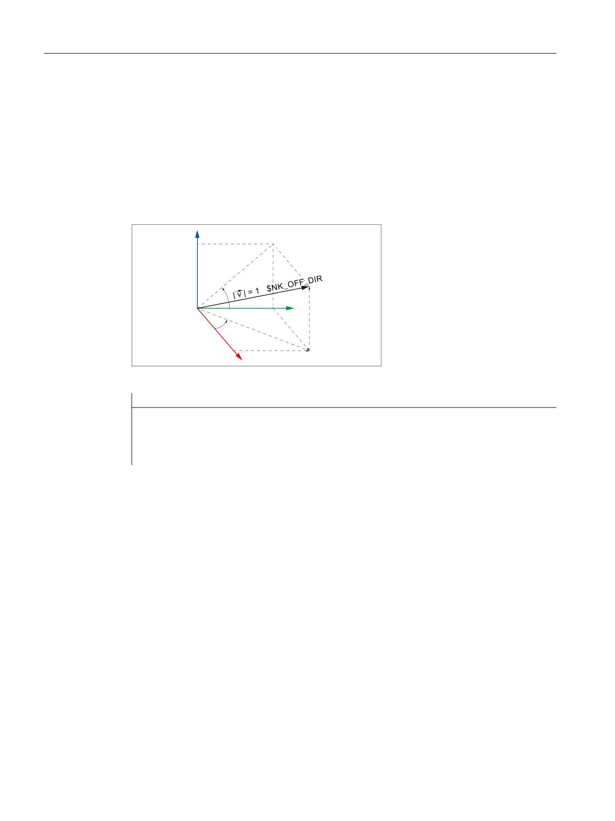
; The linear axis of the 9th element moves along the direction vector. The direction vector is the
unit vector (1; 0; 0), rotated around Z with γ=90° in the X/Y plane, and around X with α=10° in
the Y/Z plane referred to the world coordinate system. The following values result from this for
the individual components (x, y, z) of the direction vector:
• x = cos(γ) * cos(α) = cos(90) * cos(10) = 0.0
• y = sin(γ) * cos(α) = sin(90) * cos(10) ≈ 0.985
• z = sin(α) = sin(10) ≈ 0.174
=
˞
<
]
ˠ
[
;
\
Figure 5-6
Direction vector, general
Program code
Comment
; 9th kinematic element
N100 $NK_OFF_DIR[8,0] = COS(90)*COS(10)
; 0 = X component
N110 $NK_OFF_DIR[8,1] = SIN(90)*COS(10)
; 1 = Y component
N120 $NK_OFF_DIR[8,2] = SIN(10)
; 2 = Z component
$NK_AXIS
Function
The name of the machine axis (MD10000 $MN_AXCONF_MACHAX_NAME_TAB) that is to be
assigned to the element should be entered in the system variable.
The output coordinate system of the element results from the input coordinate system offset by
the current position setpoint of the machine axis in the MCS and the offset specified in
$NK_A_OFF. The position setpoint of the machine axis contains all the active work offsets and
corrections.
In accordance with the AXIS_LIN type entered in $NK_TYPE, the machine axis must be a linear
axis:
MD30300 $MA_IS_ROT_AX = 0
Syntax
$NK_AXIS[<n>] = <name>
Basic functions
416
Function Manual, 10/2020, 6FC5397-2GP40-0BA1
Kinematic chain
5.2 Commissioning
Meaning
$NK_AXIS:
Machine axis name
Data type:
STRING
Range of values:
Machine axis name
Default value:
"" (empty string)
<n>:
System variable or element index
Data type:
INT
Range of values:
0, 1, 2, ... ($MN_MM_MAXNUM_KIN_CHAIN_ELEM - 1)
<value>:
Machine axis name
Data type:
STRING
Range of values:
Machine axis names
Example
The 9th kinematic element is assigned the machine axis with the name V1 as linear axis.
Program code
Comment
N100 $NK_AXIS[8] = "V1"
; 9th kin. element
; axis = machine axis V1
$NK_A_OFF
Function
An additional work offset can be entered in the system variable for the assigned machine axis
($NK_AXIS). This work offset is only effective within the kinematic chain.
Syntax
$NK_A_OFF[<n>] = <value>
Meaning
$NK_A_OFF:
Work offset
Data type:
REAL
Range of values:
- max. REAL value ≤ x ≤ ± max. REAL value
Default value:
0.0
<n>:
System variable or element index
Data type:
INT
Range of values:
0, 1, 2, ... ($MN_MM_MAXNUM_KIN_CHAIN_ELEM - 1)
<value>:
Offset value
Data type:
REAL
Range of values:
- max. REAL value ≤ x ≤ ± max. REAL value
Example
The linear axis zero point of the 9th kinematic element is moved by 30.0 mm compared to the
modelled kinematics.
Basic functions
Function Manual, 10/2020, 6FC5397-2GP40-0BA1
417

Kinematic chain
5.2 Commissioning
The unit in which the numerical value is interpreted depends on the current input system (inch/
metric).
Program code
Comment
N100 $NK_A_OFF[8] = 30.0
; 9th kin. element
; Work offset = 30.0 mm
5.2.3.7
Type-dependent variables for $NK_TYPE = "AXIS_ROT"
$NK_OFF_DIR
Function
The direction vector around which the rotary axis $NK_AXIS assigned to the element rotates,
should be entered in the system variable. The output coordinate system is therefore calculated
from the input coordinate system, rotated by the current position value of the rotary axis and the
offset specified in $NK_A_OFF around the direction vector $NK_OFF_DIR.
Supplementary conditions:
• The direction vector must be specified as an absolute value, i.e. in relation to the world
coordinate system.
• The direction vector must be specified so that, in accordance with the "right-hand rule", the
thumb points in the direction of the vector when the rotary axis turns in the positive
direction.
• The absolute value of the direction vector must be greater than 1*10-6.
Note
Spindle
If the assigned machine axis is a spindle, its position is taken into account in different ways
specific to the function:
• Collision avoidance: Indeterminate position
• Kinematic transformation: depending on the setting in $NT_CNTRL, bit 1-3
- Bit x == 0 → indeterminate position
- Bit x == 1 → current position value + $NK_A_OFF,
Syntax
$NK_OFF_DIR[<n>,<k>] = <value>
Meaning
$NK_OFF_DIR:
Direction vector (X; Y; Z)
Data type:
REAL
Range of values:
Direction vector: 1*10-6 < |Vector | ≤ max. REAL value
Default value:
(0.0, 0.0, 0.0)
Basic functions
418
Function Manual, 10/2020, 6FC5397-2GP40-0BA1
Kinematic chain
5.2 Commissioning
<n>:
System variable or element index
Data type:
INT
Range of values:
0, 1, 2, ... ($MN_MM_MAXNUM_KIN_CHAIN_ELEM - 1)
<k>:
Coordinate index
Data type:
INT
Range of values:
0: X coordinate (abscissa)
1: Y coordinate (ordinate)
2: Z coordinate (applicate)
<value>:
Coordinate value
Data type:
REAL
Range of values:
- max. REAL value ≤ x ≤ + max. REAL value
Example
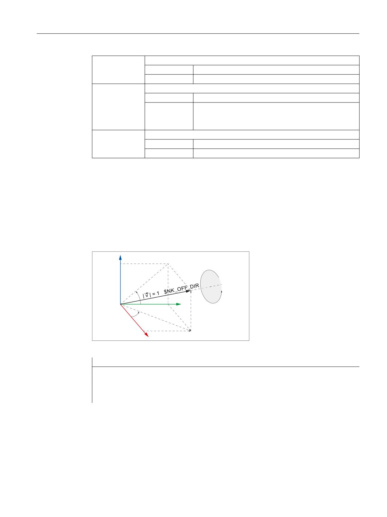
The rotary axis of the 9th element rotates around the direction vector. The direction vector is the
unit vector (1; 0; 0), rotated around Z with γ=90° in the X/Y plane, and around X with α=10° in
the Y/Z plane referred to the world coordinate system. The following values result from this for
the individual components (x, y, z) of the direction vector:
• x = cos(γ) * cos(α) = cos(90) * cos(10) = 0.0
• y = sin(γ) * cos(α) = sin(90) * cos(10) ≈ 0.985
• z = sin(α) = sin(10) ≈ 0.174
=
˞
<
]
ˠ
[
;
\
Figure 5-7
Direction vector, general
Program code
Comment
; 9th kinematic element
N100 $NK_OFF_DIR[8,0] = COS(90)*COS(10)
; 0 = X component
N110 $NK_OFF_DIR[8,1] = SIN(90)*COS(10)
; 1 = Y component
N120 $NK_OFF_DIR[8,2] = SIN(10)
; 2 = Z component
$NK_AXIS
Function
The name of the machine axis (MD10000 $MN_AXCONF_MACHAX_NAME_TAB) that is to be
assigned to the element should be entered in the system variable.
Basic functions
Function Manual, 10/2020, 6FC5397-2GP40-0BA1
419

Kinematic chain
5.2 Commissioning
The output coordinate system of the element results from the input coordinate system rotated
through the current position setpoint of the machine axis in the MCS and the offset specified in
$NK_A_OFF. The position setpoint of the machine axis contains all the active work offsets and
corrections.
The machine axis type must correspond to the type entered in $NK_TYPE:
In accordance with the AXIS_ROT type entered in $NK_TYPE, the machine axis must be a rotary
axis:
MD30300 $MA_IS_ROT_AX = 1
Syntax
$NK_AXIS[<n>] = <name>
Meaning
$NK_AXIS:
Machine axis name
Data type:
STRING
Range of values:
Machine axis name
Default value:
"" (empty string)
<n>:
System variable or element index
Data type:
INT
Range of values:
0, 1, 2, ... ($MN_MM_MAXNUM_KIN_CHAIN_ELEM - 1)
<value>:
Machine axis name
Data type:
STRING
Range of values:
Machine axis names
Example
The 9th kinematic element is assigned the machine axis with the name B1 as rotary axis.
Program code
Comment
N100 $NK_AXIS[8] = "B1"
; 9th kin. element
; axis = machine axis B1
$NK_A_OFF
Function
An additional work offset can be entered in the system variable for the assigned machine axis
($NK_AXIS). This work offset is only effective within the kinematic chain.
Syntax
$NK_A_OFF[<n>] = <value>
Basic functions
420
Function Manual, 10/2020, 6FC5397-2GP40-0BA1

Kinematic chain
5.2 Commissioning
Meaning
$NK_A_OFF:
Work offset
Data type:
REAL
Range of values:
- max. REAL value ≤ x ≤ ± max. REAL value
Default value:
0.0
<n>:
System variable or element index
Data type:
INT
Range of values:
0, 1, 2, ... ($MN_MM_MAXNUM_KIN_CHAIN_ELEM - 1)
<value>:
Offset value
Data type:
REAL
Range of values:
- max. REAL value ≤ x ≤ ± max. REAL value
Example
The rotary axis zero point of the 9th kinematic elements is moved through 30.0° compared to
the modelled kinematics.
Program code
Comment
N100 $NK_A_OFF[8] = 30.0
; 9th kin. element
; Work offset = 30.0°
5.2.3.8
Type-dependent variables for $NK_TYPE = "ROT_CONST"
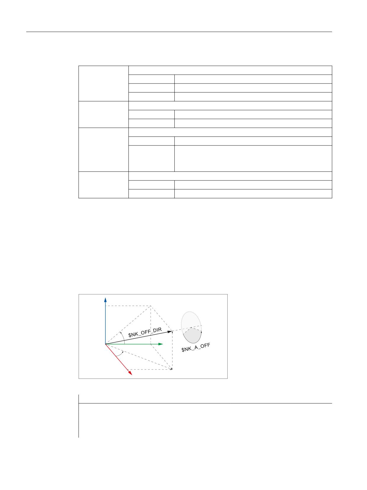
$NK_OFF_DIR
Function
The direction vector around which the constant rotation is performed should be entered in the
system variable. The output coordinate system is therefore calculated from the input coordinate
system, rotated through the angle specified in $NK_A_OFF around the direction vector
$NK_OFF_DIR.
Supplementary conditions:
• The direction vector must be specified as an absolute value, i.e. in relation to the world
coordinate system.
• The direction vector must be specified so that, in accordance with the "right-hand rule", the
thumb points in the direction of the vector when the rotary axis turns in the positive
direction.
• The absolute value of the direction vector must be greater than 1*10-6.
Syntax
$NK_OFF_DIR[<n>,<k>] = <value>
Basic functions
Function Manual, 10/2020, 6FC5397-2GP40-0BA1
421
Kinematic chain
5.2 Commissioning
Meaning
$NK_OFF_DIR:
Direction vector (X; Y; Z)
Data type:
REAL
Range of values:
Direction vector: 1*10-6 < |Vector | ≤ max. REAL value
Default value:
(0.0, 0.0, 0.0)
<n>:
System variable or element index
Data type:
INT
Range of values:
0, 1, 2, ... ($MN_MM_MAXNUM_KIN_CHAIN_ELEM - 1)
<k>:
Coordinate index
Data type:
INT
Range of values:
0: X coordinate (abscissa)
1: Y coordinate (ordinate)
2: Z coordinate (applicate)
<value>:
Coordinate value
Data type:
REAL
Range of values:
- max. REAL value ≤ x ≤ + max. REAL value
Example
The output coordinate system of the 9th Elements therefore arises from the input coordinate
system, rotated through the angle specified in $NK_A_OFF around the direction vector. The
direction vector is the unit vector (1; 0; 0), rotated around Z with γ=90° in the X/Y plane, and
around X with α=10° in the Y/Z plane referred to the world coordinate system. The following
values result from this for the individual components (x, y, z) of the direction vector:
• x = cos(γ) * cos(α) = cos(90) * cos(10) = 0.0
• y = sin(γ) * cos(α) = sin(90) * cos(10) ≈ 0.985
• z = sin(α) = sin(10) ≈ 0.174
=
˞
<
]
ˠ
[
;
\
Figure 5-8
ROT_CONST
Program code
Comment
; 9th kinematic element
N100 $NK_OFF_DIR[8,0] = COS(90)*COS(10)
; 0 = X component
N110 $NK_OFF_DIR[8,1] = SIN(90)*COS(10)
; 1 = Y component
N120 $NK_OFF_DIR[8,2] = SIN(10)
; 2 = Z component
Basic functions
422
Function Manual, 10/2020, 6FC5397-2GP40-0BA1

Kinematic chain
5.2 Commissioning
$NK_A_OFF
Function
The angle through which the output coordinate system is rotated compared with the input
coordinate system around the direction vector $NK_OFF_DIR should be entered in the system
variable.
Syntax
$NK_A_OFF[<n>] = <value>
Meaning
$NK_A_OFF:
Angle of rotation
Data type:
REAL
Range of values:
- max. REAL value ≤ x ≤ + max. REAL value
Default value:
0.0
<n>:
System variable or element index
Data type:
INT
Range of values:
0, 1, 2, ... ($MN_MM_MAXNUM_KIN_CHAIN_ELEM - 1)
<value>:
Angle
Data type:
REAL
Range of values:
- max. REAL value ≤ x ≤ + max. REAL value
Example
The angle of rotation of the 9th kinematic element is 30.0°.
Program code
Comment
N100 $NK_A_OFF[8] = 30.0
; 9th kin. element
; Angle of rotation = 30.0°
5.2.3.9
Type-dependent variables for $NK_TYPE = "OFFSET"
$NK_OFF_DIR
Function
The offset vector by which the output coordinate system is moved compared to the input
coordinate system should be entered in the system variable.
The offset vector must be specified as an absolute value, i.e. in relation to the world coordinate
system.
Syntax
$NK_OFF_DIR[<n>,<k>] = <value>
Basic functions
Function Manual, 10/2020, 6FC5397-2GP40-0BA1
423
Kinematic chain
5.2 Commissioning
Meaning
$NK_OFF_DIR:
Offset vector (X; Y; Z)
Data type:
REAL
Range of values:
(- max. REAL value) ≤ x ≤ (+ max. REAL value)
Default value:
(0.0, 0.0, 0.0)
<n>:
System variable or element index
Data type:
INT
Range of values:
0, 1, 2, ... ($MN_MM_MAXNUM_KIN_CHAIN_ELEM - 1)
<k>:
Coordinate index
Data type:
INT
Range of values:
0: X coordinate (abscissa)
1: Y coordinate (ordinate)
2: Z coordinate (applicate)
<value>:
Coordinate value
Data type:
REAL
Range of values:
(- max. REAL value) ≤ x ≤ (+ max. REAL value)
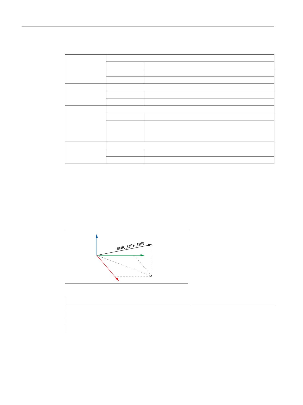
Example
The output coordinate system of the 9th element is obtained from the input coordinate system,
offset through the offset vector (x, y, z) with the following coordinates referred to the world
coordinate system:
• x = 10.0
• y = 20.0
• z = 30.0
=
<
]
[
;
\
Figure 5-9
Offset vector
Program code
Comment
; 9th kinematic element
N100 $NK_OFF_DIR[8,0] = 10.0
; 0 = X component
N110 $NK_OFF_DIR[8,1] = 20.0
; 1 = Y component
N120 $NK_OFF_DIR[8,2] = 30.0
; 2 = Z component
Basic functions
424
Function Manual, 10/2020, 6FC5397-2GP40-0BA1
Kinematic chain
5.2 Commissioning
5.2.3.10
Type-dependent variables for $NK_TYPE = "SWITCH"
$NK_SWITCH_INDEX
Function
The switch is emulated using system variables $NK_SWITCH_INDEX and $NK_SWITCH_POS (see
the following paragraph)
Index i must be entered in $NK_SWITCH_INDEX, with which the switch is closed and opened via
system variable $NK_SWITCH[<i>].
Syntax
$NK_SWITCH_INDEX[<n>] = <i>
Meaning
$NK_SWITCH_
Index i, via which the switch is addressed using system variable $NK_SWITCH[<i>]
INDEX:
Data type:
INT
Range of values:
-1, 0, 1, 2, ... ($MN_MAXNUM_KIN_SWITCHES - 1)
-1: The state of the switch is always CLOSED
Default value:
-1
<n>:
System variable or element index
Data type:
INT
Range of values:
0, 1, 2, ... ($MN_MM_MAXNUM_KIN_CHAIN_ELEM - 1)
<i>:
Index value
Data type:
INT
Example
The 9th element of the kinematic chain is a switch, which is activated by system variable
$NK_SWITCH[ 2 ].
Program code
Comment
; 9th element
N100 $NK_SWITCH_INDEX[8] = 2
; Index 2
$NK_SWITCH_POS
Function
A switch is emulated by system variables $NK_SWITCH_INDEX (see the previous paragraph) and
$NK_SWITCH_POS.
In $NK_SWITCH_POS, value p (close value) should be entered, where the switch is brought into
the CLOSED position by system variable $NK_SWITCH[<i>].
Basic functions
Function Manual, 10/2020, 6FC5397-2GP40-0BA1
425

Kinematic chain
5.2 Commissioning
Independent of $NK_SWITCH[<i>], the switch has the following states:
• CLOSED: The close value p of the switch, specified in $NK_SWITCH_POS is the same as the
actual value of $NK_SWITCH[<i>].
$NK_SWITCH_POS[<n>] == $NK_SWITCH[<i>]
The previous element of the kinematic chain is connected with the output, i.e. the following
element of the switch specified in $NK_NEXT.
• OPEN: The close value of the switch, specified in $NK_SWITCH_POS, is not the same as the
actual value of $NK_SWITCH[<i>].
$NK_SWITCH_POS[<n>] ≠ $NK_SWITCH[<i>]
The previous element of the kinematic chain is notconnected with the output, i.e. the
following element of the switch specified in $NK_NEXT.
The close value can be freely selected.
Note
Parallel element $NK_PARALLEL
The connection to a parallel element specified in $NK_PARALLEL is not influenced by the switch.
This means that the previous element is always connected to the element in the branch parallel
with the switch.
Syntax
$NK_SWITCH_POS[<n>] = <p>
Meaning
$NK_SWITCH_
Close value
POS:
Data type:
INT
Range of values:
0 ≤ x ≤ positive max. INT value
Default value:
0
<n>:
System variable or element index
Data type:
INT
Range of values:
0, 1, 2, ... ($MN_MM_MAXNUM_KIN_CHAIN_ELEM - 1)
<p>:
Value for switch position CLOSED
Data type:
INT
Example
The 9th element of the kinetic chain is a switch, which is closed if $NK_SWITCH[ 3 ] == 1
Program code
Comment
; 9th element
N110 $NK_SWITCH_POS[8] = 1
; switch position = 1
See also
$NK_SWITCH (Page 427)
$MN_MAXNUM_KIN_SWITCHES (Page 409)
Basic functions
426
Function Manual, 10/2020, 6FC5397-2GP40-0BA1
Kinematic chain
5.2 Commissioning
$MN_MM_MAXNUM_KIN_CHAIN_ELEM (Page 409)
5.2.3.11
$NK_SWITCH
Function
The switch variable comprises an array of switch positions i. The actual switch positions p should
be entered in this array.
Function
To parameterize (Page 425) a switchi in a kinematic chain, switchiwith index i must be connected
to the switch variable and its switch position p for the CLOSED state assigned to it.
$NK_SWITCH_INDEX[<n>] = <i>
$NK_SWITCH_POS[<n>]
= <p>
Switchi can then be closed and opened via index i of the switch variable:
Close: $NK_SWITCH[<i>] = <p>
Open: $NK_SWITCH[<i>] ≠ <p>
As many switches as required can be connected with an index of the switch variable.
Syntax
$NK_SWITCH[<i>] = <p>
Meaning
$NK_SWITCH<i>:
Switch variable with switch positions i
Data type:
INT
Value range:
-1 ≤x ≤ positive max. INT value
Note
-1: Initial state OPEN
<i>:
Switch index
Data type:
INT
Range of values:
0, 1, 2, ... (MD18882 $MN_MM_MAX_NUM_KIN_SWITCHES - 1)
<p>:
Switch setting
Data type:
INT
Value range:
-1 ≤x ≤ positive max. INT value
-1: Initial state OPEN
Basic functions
Function Manual, 10/2020, 6FC5397-2GP40-0BA1
427
Kinematic chain
5.3 Programming
Example
The 9th kinematic element is assigned the name "B axis":
Program code
Comment
N100 $NK_SWITCH[3] = 1
; actual switch position
; for switch [3] = 1
5.3
Programming
5.3.1
Deletion of components (DELOBJ)
The DELOBJ() function "deletes" components by resetting the assigned system variables to
their default values:
• Elements from kinematic chains
• Protection areas, protection area elements and collision pairs
• Transformation data
Syntax
[<RetVal>=] DELOBJ(<CompType>[,,,<NoAlarm>)])
[<RetVal>=] DELOBJ(<CompType>,<Index1>[,,<NoAlarm>])
[<RetVal>=] DELOBJ(<CompType>[,<Index1>][,<Index2>][,<NoAlarm>])
Basic functions
428
Function Manual, 10/2020, 6FC5397-2GP40-0BA1

Kinematic chain
5.3 Programming
Meaning
DELOBJ:
Deletion of elements from kinematic chains, protection areas, protection area ele-
ments, collision pairs and transformation data
<CompType>:
Component type to be deleted
Data type:
STRING
Value: "KIN_CHAIN_ELEM"
Meaning: System variables of all kinematic elements: $NK_...
Value: "KIN_CHAIN_SWITCH"
Meaning: System variable $NK_SWITCH[<i>]
Value: "KIN_CHAIN_ALL"
Meaning: All kinematic elements and switches.
Is the same as the successive call of DELOBJ with "KIN_CHAIN_ELEM" and
"KIN_CHAIN_SWITCH"
Value: "PROT_AREA"
Meaning: System variables of the protection areas:
• $NP_PROT_NAME
• $NP_CHAIN_NAME
• $NP_CHAIN_ELEM
• $NP_1ST_PROT
Value: "PROT_AREA_ELEM"
Meaning: System variables of the protection area elements of machine protection
areas and/or automatic tool protection areas:
• $NP_NAME
• $NP_NEXT
• $NP_NEXTP
• $NP_COLOR
• $NP_D_LEVEL
• $NP_USAGE
• $NP_TYPE
• $NP_FILENAME
• $NP_PARA
• $NP_OFF
• $NP_DIR
• $NP_ANG
Value: "PROT_AREA_COLL_PAIRS"
Meaning: System variables of the collision pairs:
• $NP_COLL_PAIR
• $NP_SAFETY_DIST
Value: "PROT_AREA_ALL"
Meaning: All protection areas, protection area elements and collision pairs (system
variable $NP_... )
Is the same as the successive call of DELOBJ with "PROT_AREA," "PROT_AREA_ELEM,"
and "PROT_AREA_COLL_PAIRS"
Value: "TRAFO_DATA"
Meaning: System variables of all transformations $NT_...
Basic functions
Function Manual, 10/2020, 6FC5397-2GP40-0BA1
429

Kinematic chain
5.3 Programming
<Index1>:
Index of the first component to be deleted (optional)
Data type:
INT
Default value:
-1
Value range:
-1 ≤ x ≤ (maximum number of configured components -1)
Value
Meaning
0, 1, 2,
Index of the component to be deleted
-1
All components of the specified type are deleted. <Index2> is not
evaluated.
<Index2>:
Index of the last components to be deleted (optional)
If <Index2> is not programmed, only the system variables of the component refer-
enced in <Index1> are deleted.
Data type:
INT
Default value:
Only the system variables of the component referenced in <In-
dex1> are deleted.
Value range:
<Index1> < x ≤ (max. number of configured components -1)
<NoAlarm>:
Alarm suppression (optional)
Data type:
BOOL
Default value:
FALSE
Value
Meaning
FALSE
In the event of an error (<RetVal> < 0), program processing is stop-
ped and an alarm displayed.
TRUE
In the event of an error, the program processing is not stopped and
no alarm displayed.
Application: User-specific reaction corresponding to the return val-
ue
<RetVal>:
Function return value
Data type:
INT
Value range:
0, -1, -2, ... -7
Value
Meaning
0
No error occurred
-1
Call of the function without parameters. At least parameter
<CompType> must be specified.
-2
<CompType> identifies an unknown component
-3
<Index1> is less than -1
-4
<Index1> is greater than the configured number of components
-5
<Index1> has a value not equal to -1 when deleting a compo-
nent group
-6
<Index2> is less than <Index1>
-7
<Index2> is greater than the configured number of components
-8
Insufficient write permission
Basic functions
430
Function Manual, 10/2020, 6FC5397-2GP40-0BA1

Kinematic chain
5.3 Programming
5.3.2
Index determination by means of names (NAMETOINT)
User-specific names are entered in the system variable arrays of type STRING. Based on the
identifier of the system variables and the name, the NAMETOINT() function determines the
index value belonging to the name under which it is stored in the system variable array.
Syntax
<RetVal> = NAMETOINT(<SysVar>,<Name>[,<NoAlarm>])
Meaning
NAMETOINT:
Determining the system variable index
<SysVar>:
Name of the system variable array of typeSTRING
Data type:
STRING
Range of val-
Name of all NC system variable arrays of type STRING
ues:
<Name>:
Character string or name for which the system variable index is to be determined.
Data type:
STRING
<NoAlarm>:
Alarm suppression (optional)
Data type:
BOOL
Default value:
FALSE
Value
Meaning
TRUE
In the event of an error, the program processing is not stopped and
no alarm displayed.
Application: User-specific reaction corresponding to the return val-
ue
FALSE
In the event of an error (<RetVal> < 0), program processing is stop-
ped and an alarm displayed.
<RetVal>:
System variable index or error message
Data type:
INT
Range of val-
-1 ≤ x ≤ (max. number of configured components -1)
ues:
Value
Meaning
≥ 0
The sought name has been found under the specified system var-
iable index.
-1
The sought name has not been found or an error has occurred.
Example
Program code
Comment
DEF INT INDEX
$NP_PROT_NAME[27]="Cover"
INDEX = NAMETOINT("$NP_PROT_NAME","Cover")
; INDEX == 27
Basic functions
Function Manual, 10/2020, 6FC5397-2GP40-0BA1
431
Kinematic chain
5.4 Example
5.4
Example
5.4.1
Specifications
General Information
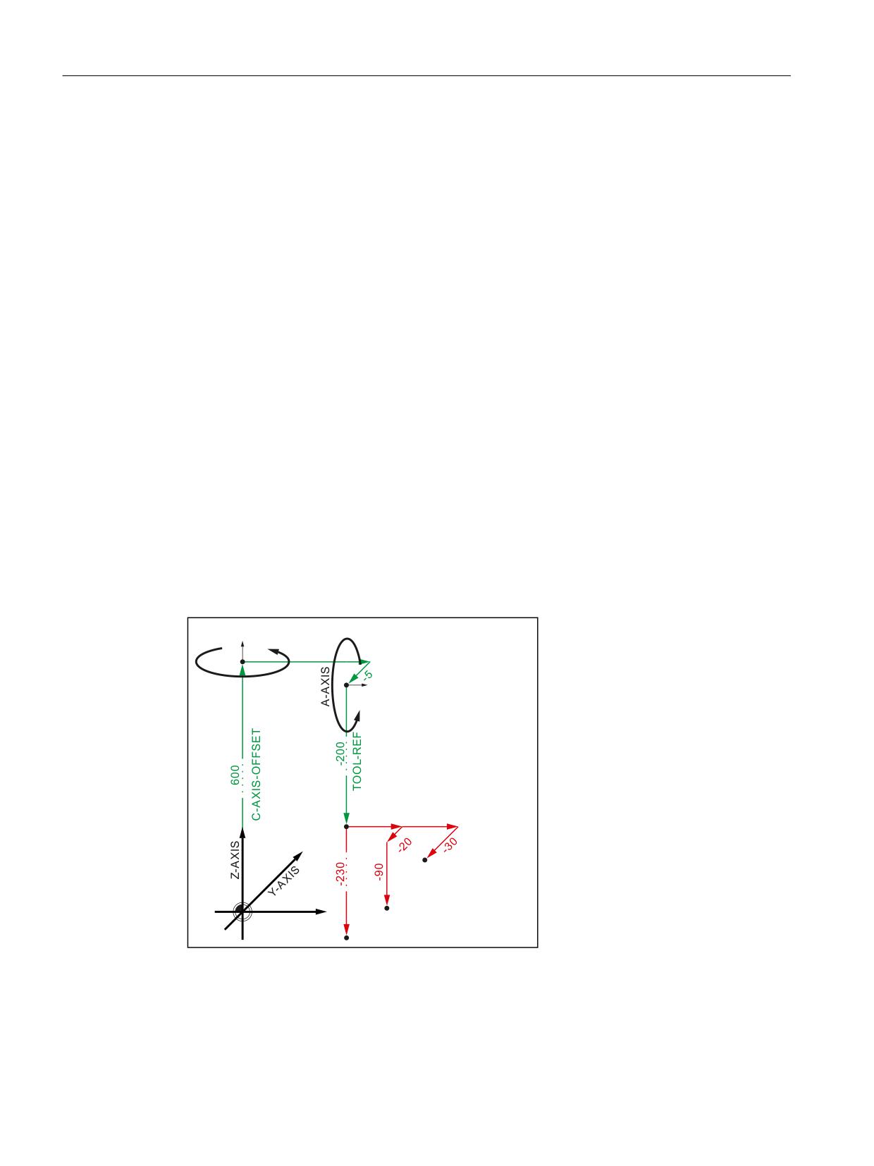
The principle approach when parameterizing a kinematic chain with three switches using a part
program is shown using as example a 5-axis machine with three different tool heads, which are
used alternately. All of the system variables, relevant for kinematic chain, are written to the part
program:
• Kinematic chain $NK_...
Option and machine data
The following option and machine data must be set for the example:
• MD19830 $ON_COLLISION_MASK.Bit 0 = 1
• MD18880 $MN_MM_MAXNUM_KIN_CHAIN_ELEM = 15
Kinematic chain
Schematic representation of the machine kinematics
& $ $;,6
2))6(7
& $
;,6
6
+($'
6
+($'
; $;,6
6
+($'
Basic functions
432
Function Manual, 10/2020, 6FC5397-2GP40-0BA1
Kinematic chain
5.4 Example
Elements of the kinematic chain
5RRW
; $;,6
<$;,6
= $;,6
& $;,6
& $;,6
2))6(7
$;,6B/,1
$;,6B/,1
$;,6B/,1
2))
$;,6B527
2))6(7
'2&.B3B
+($'
6:,7&+
2))6(7
'2&.B3B
+($'
6:,7&+
2))6(7
& $ $;,6
$ $;,6
722/ 5()
'2&.B3B
+($'
2))
$;,6B527
2))6(7
6:,7&+
2))6(7
2))6(7
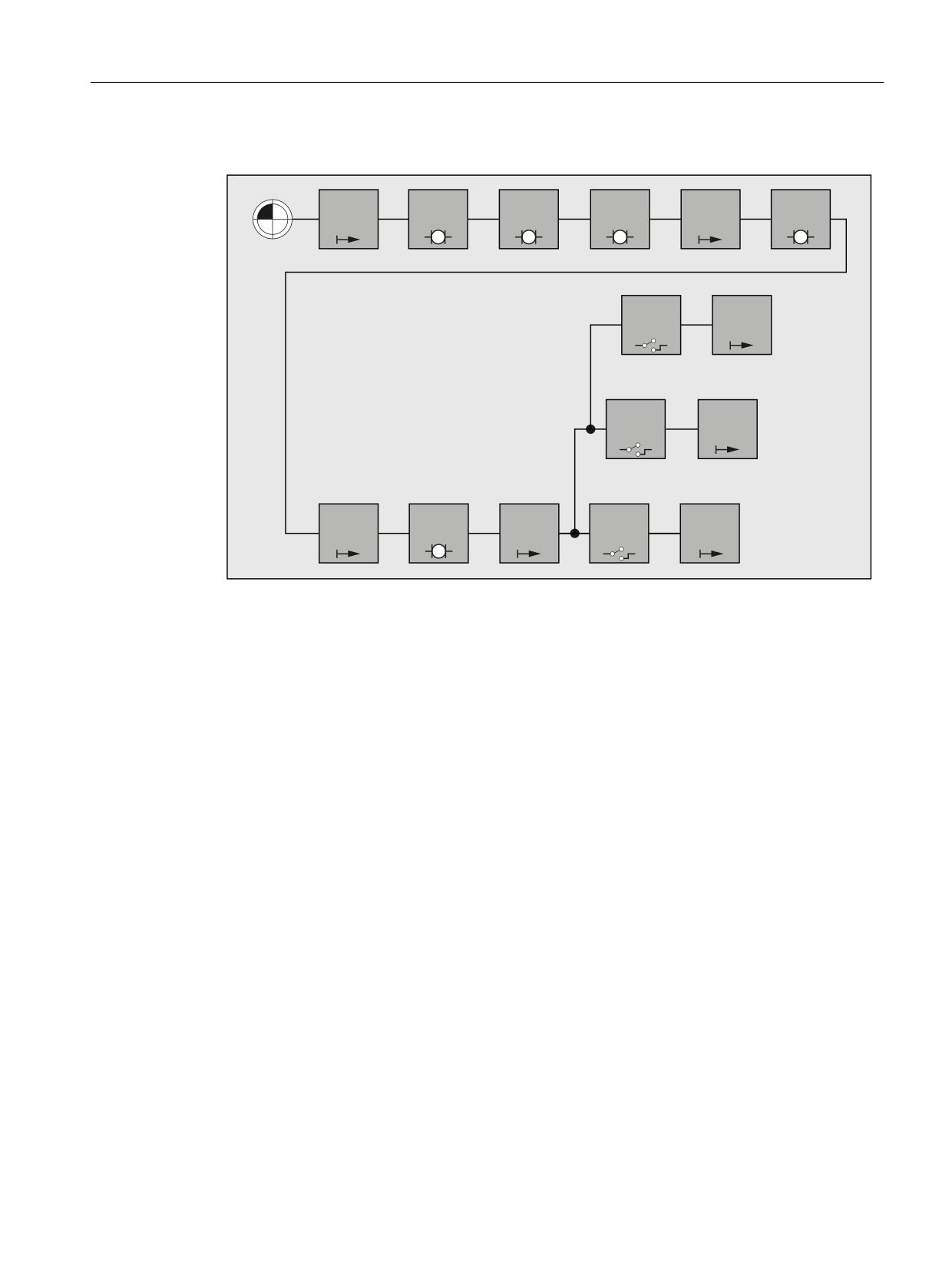
The kinematic chain starts with an element of the type "Offset". When completely
parameterizing the collision avoidance, these are assigned to all static protection areas of the
machine
The offset element is followed by the kinematic elements of the linear machine axes X, Y and Z
- as well as the offset and kinematic elements of rotary axes C and A.
The offset element for the reference point of the tool heads is followed by three switches to
switch on and switch off the tool heads. As a result of $NK_INDEX = 3 all three switches refer to
the same switch variable $NK_SWITCH[ 3 ]. As a result of the different switch positions (1, 2, 3),
only the subchain of the active tool head is active.
Basic functions
Function Manual, 10/2020, 6FC5397-2GP40-0BA1
433
Kinematic chain
5.4 Example
5.4.2
Part program of the machine model
Program code
;===========================================================
; Definitions
;===========================================================
N10 DEF INT KIE_CNTR ; COUNTER FOR ELEMENTS OF THE KIN. CHAINS
N20 DEF INT RETVAL
;
;===========================================================
; Initialization of collision data
;===========================================================
; Reset all parameters to their initial values:
N30 RETVAL = DELOBJ("KIN_CHAIN_ELEM")
N40 KIE_CNTR = 0
;
;===========================================================
; Kinematic chain
;===========================================================
; KE1: OFFSET: Root
; ----------------------------------------------------------
N50 $NK_TYPE[KIE_CNTR] = "OFFSET"
N60 $NK_NAME[KIE_CNTR] = "ROOT"
N70 $NK_NEXT[KIE_CNTR] = "X-AXIS"
N80 KIE_CNTR = KIE_CNTR + 1
;
; ----------------------------------------------------------
; Kinematic element: LINEAR AXIS: X axis
; ----------------------------------------------------------
N90 $NK_TYPE[KIE_CNTR] = "AXIS_LIN"
N100 $NK_NAME[KIE_CNTR] = "X-AXIS"
N110 $NK_NEXT[KIE_CNTR] = "Y-AXIS"
N120 $NK_AXIS[KIE_CNTR] = "X1"
;
N130 $NK_OFF_DIR[KIE_CNTR,0] = 1.0
; X
N140 KIE_CNTR = KIE_CNTR + 1
;
; ----------------------------------------------------------
; Kinematic element: LINEAR AXIS: Y axis
; ----------------------------------------------------------
N150 $NK_TYPE[KIE_CNTR] = "AXIS_LIN"
N160 $NK_NAME[KIE_CNTR] = "Y-AXIS"
N170 $NK_NEXT[KIE_CNTR] = "Z-AXIS"
N180 $NK_AXIS[KIE_CNTR] = "Y1"
;
N190 $NK_OFF_DIR[KIE_CNTR,1] = 1.0
; Y
N200 KIE_CNTR = KIE_CNTR + 1
;
; ----------------------------------------------------------
; Kinematic element: LINEAR AXIS: Z axis
; ----------------------------------------------------------
N210 $NK_TYPE[KIE_CNTR] = "AXIS_LIN"
N220 $NK_NAME[KIE_CNTR] = "Z-AXIS"
N230 $NK_NEXT[KIE_CNTR] = "C-AXIS-OFFSET"
N240 $NK_AXIS[KIE_CNTR] = "Z1"
;
Basic functions
434
Function Manual, 10/2020, 6FC5397-2GP40-0BA1
Kinematic chain
5.4 Example
Program code
N250 $NK_OFF_DIR[KIE_CNTR,2] = 1.0
; Z
N260 KIE_CNTR = KIE_CNTR + 1
;
; ----------------------------------------------------------
; Kinematic element: OFFSET: C axis
; ----------------------------------------------------------
N270 $NK_TYPE[KIE_CNTR] = "OFFSET"
N280 $NK_NAME[KIE_CNTR] = "C-AXIS-OFFSET"
N290 $NK_NEXT[KIE_CNTR] = "C-AXIS"
;
N300 $NK_OFF_DIR[KIE_CNTR,2] = 600.0
; Z direction
N310 KIE_CNTR = KIE_CNTR + 1 ;
;
; ----------------------------------------------------------
; Kinematic element: ROTARY AXIS: C axis
; ----------------------------------------------------------
N320 $NK_TYPE[KIE_CNTR] = "AXIS_ROT"
N330 $NK_NAME[KIE_CNTR] = "C-AXIS"
N340 $NK_NEXT[KIE_CNTR] = "C-A-OFFSET"
N350 $NK_AXIS[KIE_CNTR] = "C1"
;
N360 $NK_OFF_DIR[KIE_CNTR,2] = 1.0
; Z direction
N370 KIE_CNTR = KIE_CNTR + 1
;
; ----------------------------------------------------------
; Kinematic element: OFFSET: C-A axis
; ----------------------------------------------------------
N380 $NK_TYPE[KIE_CNTR] = "OFFSET"
N390 $NK_NAME[KIE_CNTR] = "C-A-OFFSET"
N400 $NK_NEXT[KIE_CNTR] = "A-AXIS"
;
N410 $NK_OFF_DIR[KIE_CNTR,0] = 20.0
; X direction
N420 $NK_OFF_DIR[KIE_CNTR,1] = -5.0
; Y direction
N430 KIE_CNTR = KIE_CNTR + 1
;
; ----------------------------------------------------------
; Kinematic element: ROTARY AXIS: A axis
; ----------------------------------------------------------
N440 $NK_TYPE[KIE_CNTR] = "AXIS_ROT"
N450 $NK_NAME[KIE_CNTR] = "A-AXIS"
N460 $NK_NEXT[KIE_CNTR] = "TOOL-REF"
N470 $NK_AXIS[KIE_CNTR] = "A1"
;
N480 $NK_OFF_DIR[KIE_CNTR,0] = 1.0
; X direction
N490 KIE_CNTR = KIE_CNTR + 1
;
; ----------------------------------------------------------
; Kinematic element: OFFSET: Tool reference
; ----------------------------------------------------------
N500 $NK_TYPE[KIE_CNTR] = "OFFSET"
N510 $NK_NAME[KIE_CNTR] = "TOOL-REF"
N520 $NK_NEXT[KIE_CNTR] = "DOCKING_POINT 1"
;
N530 $NK_OFF_DIR[KIE_CNTR,2] = -200.0
; Z direction
N540 KIE_CNTR = KIE_CNTR + 1
;
Basic functions
Function Manual, 10/2020, 6FC5397-2GP40-0BA1
435
Kinematic chain
5.4 Example
Program code
; ----------------------------------------------------------
; Kinematic element: Switch 3/1
; ----------------------------------------------------------
N550 $NK_TYPE[KIE_CNTR] = "SWITCH"
N560 $NK_NAME[KIE_CNTR] = "DOCKING_POINT 1"
N570 $NK_NEXT[KIE_CNTR] = "HEAD 1"
N580 $NK_PARALLE[KIE_CNTR] = "DOCKING_POINT 2"
;
N590 $NK_SWITCH_INDEX[KIE_CNTR] = 3
; Index 3
N600 $NK_SWITCH_POS[KIE_CNTR] = 1
; switch position 1
N610 KIE_CNTR = KIE_CNTR + 1
;
; ----------------------------------------------------------
; Kinematic element: Switch 3/2
; ----------------------------------------------------------
N620 $NK_TYPE[KIE_CNTR] = "SWITCH"
N630 $NK_NAME[KIE_CNTR] = "DOCKING_POINT 2"
N640 $NK_NEXT[KIE_CNTR] = "HEAD 2"
N650 $NK_PARALLE[KIE_CNTR] = "DOCKING_POINT 3"
;
N660 $NK_SWITCH_INDEX[KIE_CNTR] = 3
; Index 3
N670 $NK_SWITCH_POS[KIE_CNTR] = 2
; switch position 2
N680 KIE_CNTR = KIE_CNTR + 1
;
; ----------------------------------------------------------
; Kinematic element: Switch 3/3
; ----------------------------------------------------------
N690 $NK_TYPE[KIE_CNTR] = "SWITCH"
N700 $NK_NAME[KIE_CNTR] = "DOCKING_POINT 3"
N710 $NK_NEXT[KIE_CNTR] = "HEAD 3"
N720 $NK_PARALLE[KIE_CNTR] = ""
N730 $NK_SWITCH_INDEX[KIE_CNTR] = 3
; Index 3
N740 $NK_SWITCH_POS[KIE_CNTR] = 3
; switch position 3
N750 KIE_CNTR = KIE_CNTR + 1
;
; ----------------------------------------------------------
; Kinematic element: OFFSET: HEAD 1
; ----------------------------------------------------------
N760 $NK_TYPE[KIE_CNTR] = "OFFSET"
N770 $NK_NAME[KIE_CNTR] = "HEAD 1"
N780 $NK_NEXT[KIE_CNTR] = ""
;
N790 $NK_OFF_DIR[KIE_CNTR,0] = 100
; X direction
N800 $NK_OFF_DIR[KIE_CNTR,1] = -30
; Y direction
N810 KIE_CNTR = KIE_CNTR + 1
;
; ----------------------------------------------------------
; Kinematic element: OFFSET: HEAD 2
; ----------------------------------------------------------
N820 $NK_TYPE[KIE_CNTR] = "OFFSET"
N830 $NK_NAME[KIE_CNTR] = "HEAD 2"
N840 $NK_NEXT[KIE_CNTR] = ""
;
N850 $NK_OFF_DIR[KIE_CNTR,2] = -230
; Z direction
N860 KIE_CNTR = KIE_CNTR + 1
;
Basic functions
436
Function Manual, 10/2020, 6FC5397-2GP40-0BA1

Kinematic chain
5.5 Data lists
Program code
; ----------------------------------------------------------
; Kinematic element: OFFSET: HEAD 3
; ----------------------------------------------------------
N870 $NK_TYPE[KIE_CNTR] = "OFFSET"
N880 $NK_NAME[KIE_CNTR] = "HEAD 3"
N890 $NK_NEXT[KIE_CNTR] = ""
;
N900 $NK_OFF_DIR[KIE_CNTR,0] = 50
; X direction
N910 $NK_OFF_DIR[KIE_CNTR,1] = -20
; Y direction
N920 $NK_OFF_DIR[KIE_CNTR,2] = -90
; Z direction
N930 KIE_CNTR = KIE_CNTR + 1
End
5.5
Data lists
5.5.1
Machine data
5.5.1.1
NC-specific machine data
Number
Identifier: $MN_
Description
16800
ROOT_KIN_ELEM_NAME
Name of the first element in the kinematic chain
18880
MM_MAXNUM_KIN_CHAIN_ELEM
Maximum number of elements for kinematic chains
18882
MM_MAX_NUM_KIN_SWITCHES
Maximum number of switches for kinematic chains
5.5.2
System variables
Identifier
Description
$NK_NAME
Name of the kinematic element
$NK_NEXT
Name of the next element in the kinematic chain
$NK_PARALLEL
Name of the first element of a parallel branching kinematic chain before the
element
$NK_TYPE
Type of the kinematic element
$NK_OFF_DIR
Depends on $NK_TYPE: Offset or direction vector
$NK_AXIS
Name of the assigned machine axis or object name
$NK_A_OFF
Work offset in the element for linear or rotary axes
$NK_SWITCH_INDEX
Index i, via which the switch is addressed using system variable
$NK_SWITCH[<i>]
$NK_SWITCH_POS
Switch position CLOSED
$NK_SWITCH
Switch variable
Basic functions
Function Manual, 10/2020, 6FC5397-2GP40-0BA1
437
Kinematic chain
5.5 Data lists
Basic functions
438
Function Manual, 10/2020, 6FC5397-2GP40-0BA1
Continuous-path mode, exact stop, LookAhead
6
6.1
Brief Description
Exact stop or exact stop mode
In exact stop traversing mode, all axes involved in the traversing motion (except axes of modal
traversing modes) are decelerated at the end of each block until they come to a standstill. The
transition to the next block occurs only when all axes involved in the traversing motion have
reached their programmed target position depending on the selected exact stop criterion.
Continuous-path mode
In the continuous-path mode, the NC attempts to keep the programmed path velocity as
constant as possible. In particular, deceleration of the path axes at the block limits of the part
program is to be avoided.
LookAhead
LookAhead is a function for optimizing the continuous path mode.
Smooth and uniform machining of workpieces is necessary to ensure a high-quality surface
finish. For this reason, path velocity variations should be avoided during machining whenever
possible. Without LookAhead, the NC only takes the traversing block immediately following the
current traversing block into consideration when determining the possible path velocity. If the
following block contains only a short path, the NC must reduce the path velocity (decelerate in
the current block) to be able to stop in time at the end of the next block, if necessary.
When the NC "looks ahead" over a configurable number of traversing blocks following the
current traversing block, a much higher path velocity can be attained under certain
circumstances because the NC now has considerably more traversing blocks and more path
available for calculation.
This has the following advantages:
• Machining with higher path velocities on average
• Improved surface quality by avoiding deceleration and acceleration
Smoothed path velocity
"Smoothing the path velocity" is a function especially for applications (such as high speed milling
in mold and die making) that require an extremely steady and consistent path velocity.
Deceleration and acceleration processes that would cause high-frequency excitation of machine
resonances are avoided with the "Smoothing the path velocity" function.
Basic functions
Function Manual, 10/2020, 6FC5397-2GP40-0BA1
439
Continuous-path mode, exact stop, LookAhead
6.1 Brief Description
This has the following advantages:
• Improved surface quality and shorter machining time by avoiding excitation of machine
resonances.
• Constant profile of path velocity and cutting rates by avoiding "unnecessary" acceleration
processes, i.e. acceleration processes that do not greatly improve the program run time.
Adaptation of the dynamic path response
In addition to "smoothing the path velocity", "dynamic path response adaptation" is another
function for avoiding high-frequency excitations of machine resonances while optimizing the
dynamic path response at the same time. To achieve this, highly frequency changes in path
velocity are automatically executed with lower jerk or acceleration values than the dynamic
response limit value parameterized in the machine data.
Thus, with low-frequency changes in the path velocity, the full dynamic response limit values
apply, whereas with high-frequency changes, only the reduced dynamic response limit values
act due to the automatic dynamic response adaptation.
Dynamic response mode for path interpolation
Optimizing the path dynamic response also includes the technology-specific dynamic response
settings which are preset for different machining technologies (including tapping, roughing,
smoothing) and can be activated in the part program by calling the respective dynamic response
mode.
Free-form surface mode
Any fluctuation in curvature or torsion leads to a change in path velocity. This generally results
in unnecessary decelerating and accelerating while machining free-form surface workpieces,
which may adversely affect the quality of the surfaces of the workpieces.
The following functions are available for machining free-form surfaces.
• "Free-form surface mode: Basic functions"
This makes the definition of the path velocity profile "less sensitive" to fluctuations in
curvature and torsion.
• "Free-form surface mode: Extension function"
This extension in standard LookAhead functionality is used to calculate the path velocity
profile while machining free-form surfaces.
The advantages of free-form surface mode lie in a more homogeneous workpiece surface and
lower machine stress levels.
Compressing linear blocks
When a workpiece design is completed with a CAD/CAM system, the CAD/CAM system generally
also compiles the corresponding part program to create the workpiece surface. To do so, most
CAD/CAM systems use linear blocks to describe even curved sections of the workpiece surface.
Many interpolation points are generally necessary to maintain the required contour accuracy.
This results in many linear blocks, typically with very short paths.
Basic functions
440
Function Manual, 10/2020, 6FC5397-2GP40-0BA1
Continuous-path mode, exact stop, LookAhead
6.2 Exact stop mode
The "Compressor function" uses polynomial blocks to perform a subsequent approximation of
the contour specified by the linear blocks. During this process, an assignable number of linear
blocks is replaced by a polynomial block.
Advantages:
• Reduction of the number of traversing blocks
• Increased path velocity
• Increased surface quality
• Continuous block transitions
Compressing short spline blocks
A spline defines a curve, which comprises 2nd or 3rd degree polynomials With spline
interpolation, the control system can generate a smooth curve characteristic from only a few
specified interpolation points of a set contour.
The advantages of the spline interpolation as compared to the linear interpolation are:
• Reduction of the number of required part program blocks for describing a curved contour.
• Soft characteristic that reduces the stress on the mechanical system, even between part
program blocks.
The disadvantages of spline interpolation as compared to linear interpolation are:
• For a spline curve no exact curve characteristic, but only a tolerance band can be specified,
within which the spline curve should lie.
As with linear interpolation, the processing of splines can produce such short blocks that the
path velocity must be reduced to enable interpolation of the spline blocks. This is also the case,
when the spline has a long, smooth curve. The "Compression of short spline blocks" function
allows you to combine these spline blocks such that the resulting block length is sufficient and
does not reduce the path velocity.
6.2
Exact stop mode
Exact stop or exact stop mode
In the exact stop traversing mode, all path axes and special axes involved in the traversing
motion that are not traversed modally, are decelerated at the end of each block until they come
to a standstill. The transition to the next block occurs only when all axes involved in the
traversing motion have reached their programmed target position depending on the selected
exact stop condition.
This results in the following response are obtained:
• The program run time is considerably longer compared to continuous path mode due to the
deceleration of the axes and the wait time until "Exact stop" status is reached for all machine
axes involved.
• In exact stop mode, undercuts can occur on the workpiece surface during machining.
Basic functions
Function Manual, 10/2020, 6FC5397-2GP40-0BA1
441
Continuous-path mode, exact stop, LookAhead
6.2 Exact stop mode
Exact stop condition
The following exact stop conditions can be set:
• "Exact stop coarse"
• "Exact stop fine"
• "Interpolator end"
Application
Exact stop mode should always be used when the programmed contour must be executed
exactly.
Activation
In a program, exact stop operation can be specified using the following commands, either modal
or for specific blocks:
Command
Meaning
G60
Exact stop operation is effective from the current modal block.
G9
Exact stop operation is effective in the current block.
Exact stop conditions - "Exact stop coarse" and "Exact stop fine"
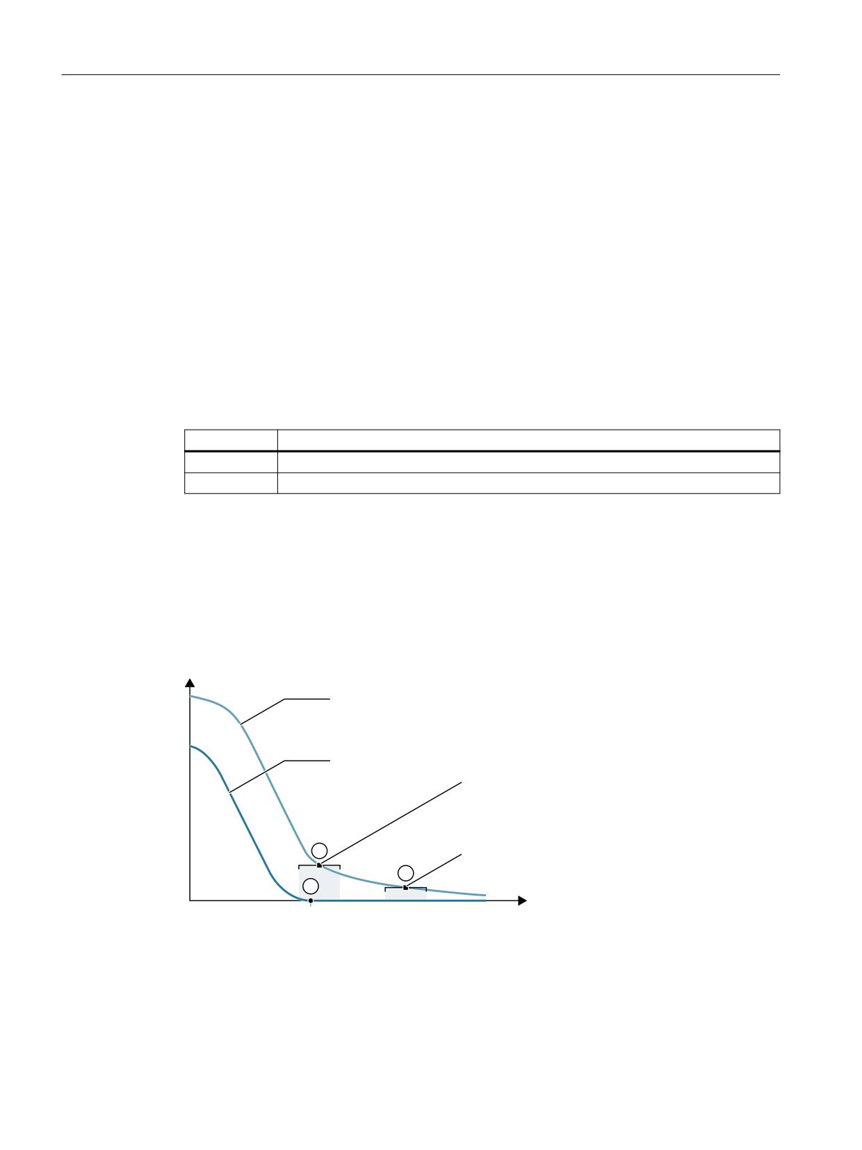
The exact stop condition "coarse" or "fine" is fulfilled by a machine axis if its current following
error is less than or equal to the tolerance range around the setpoint position, parameterized in
the machine data:
• MD36000 $MA_STOP_LIMIT_COARSE (exact stop coarse)
• MD36010 $MA_STOP_LIMIT_FINE (exact stop fine)
)ROORZLQJ HUURU
9HORFLW\ VHWSRLQW
'%
ಹ '%;
H[DFW VWRS FRDUVH
'%
ಹ '%;
H[DFW VWRS ILQH
Setpoint position
W
Figure 6-1
Tolerance window of exact stop conditions
Basic functions
442
Function Manual, 10/2020, 6FC5397-2GP40-0BA1

Continuous-path mode, exact stop, LookAhead
6.2 Exact stop mode
Note
The tolerance windows of the exact stop conditions "Exact stop coarse" and "Exact stop fine"
should be assigned in such a way that the following requirement is fulfilled:
"Exact stop coarse" > "Exact stop fine"
Exact stop condition, "Interpolator end"
With exact stop condition "Interpolator end", the block change to the next block takes place as
soon as all path axes and non-modal special axes involved in the traversing motion have reached
the position programmed in the block in terms of the setpoint value. That is, the interpolator has
executed the block.
The actual position and the following error of the relevant machine axes are not taken into
consideration for exact stop condition "Interpolator end". Thus, depending on the dynamic
response of the machine axes, this can result in a relatively large smoothing of the contour at the
block changes in comparison to the exact stop conditions "Exact stop coarse" and "Exact stop
fine".
Activating the programmable exact stop conditions
The programmable exact stop conditions are activated using the following commands:
Command
Exact stop condition
G601
Exact stop fine
G602
Exact stop coarse
G603
Interpolator end
Basic functions
Function Manual, 10/2020, 6FC5397-2GP40-0BA1
443
Continuous-path mode, exact stop, LookAhead
6.2 Exact stop mode
Block change depending on exact stop condition
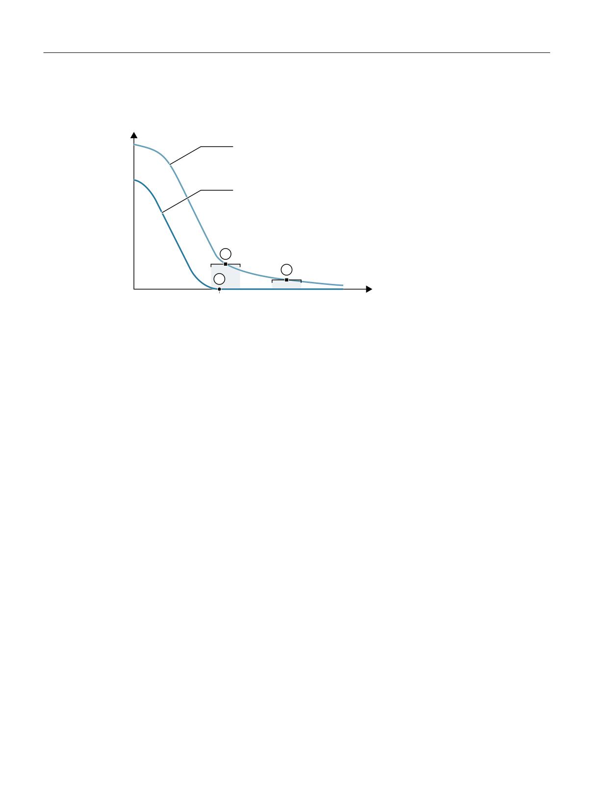
The figure below illustrates the block change timing in terms of the selected exact stop condition.
)ROORZLQJ HUURU
9HORFLW\ VHWSRLQW
Setpoint position
W
① Set position/block change points G603
② G602 MD36000 $MA_STOP_LIMIT_COARSE
③ G601 MD36010 $MA_STOP_LIMIT_FINE
Figure 6-2
Block change depending on exact stop condition
Weighting factor for exact stop conditions
A parameter set-dependent evaluation of the exact stop conditions can be specified via the
following axis-specific machine data:
MD36012 $MA_STOP_LIMIT_FACTOR[<Parameter set>] = <Value>
The evaluation factor is applied to the values of the following machine data:
• MD36000 $MA_STOP_LIMIT_COARSE
• MD36010 $MA_STOP_LIMIT_FINE
• MD36030 $MA_STANDSTILL_POS_TOL
Application examples
• Adaptation of the positioning response to different mass ratios, such as after a new gearbox
stage has been selected.
• Reduction in positioning time, depending on various machining states, such as roughing and
finishing
Parameterizable input of the effective exact stop conditions
The exact stop conditions for the commands of the 1st G group can be defined permanently. As
a consequence, programmed exact stop conditions are no longer effective.
Exact stop conditions can be set independently of one another for the following commands:
• Rapid traverse G0
• All other commands of the 1st G group
Basic functions
444
Function Manual, 10/2020, 6FC5397-2GP40-0BA1

Continuous-path mode, exact stop, LookAhead
6.2 Exact stop mode
The exact stop condition is set on a channel-for-channel basis using the following decimal-coded
machine data:
MD20550 $MC_EXACT_POS_MODE = <Z><E>
Z
E
Effective exact stop condition
0
0
Programmed exact stop condition
1
1
G601 (Exact stop window fine)
2
2
G602 (Exact stop window coarse)
3
3
G603 (Interpolator end)
E (ones position): Setting the exact stop condition für rapid traverse.
Z (tens position): Setting the exact stop condition for all other commands of the 1st G group
Example
MD20550 $MC_EXACT_POS_MODE = 02
• <E> = 2: With rapid traverse, exact stop condition G602 (exact stop window coarse) is always
active, irrespective of any programming.
• <Z> = 0: When traversing with all other commands of the 1st G group, the programmed exact
stop condition applies.
Block change behavior for block transitions from G0 ↔ non-G0 to continuous path mode
For the continuous path mode, the block change behavior between rapid traverse and non rapid
traverse blocks (G0 ↔ non-G0) can be set using the following machine data:
MD20552 $MC_EXACT_POS_MODE_G0_TO_G1 = <Value>
<Val-
Meaning
ue>
0
No additional stop at the block transition.
1
Stop at the block transition.
The behavior corresponds to G601 (exact stop window, fine)
2
Stop at the block transition.
The behavior corresponds to G602 (exact stop window, coarse)
3
Stop at the block transition.
The behavior corresponds to G603 (interpolator end)
4
No stop at the block transition.
For the continuous path mode, for block changes from G0 → non-G0, in the G0 block, the
actual value of the feedrate correction of the subsequent non-G0 block is predicatively taken
into account. Depending on the axis dynamic performance and the path length of the current
block, the block change is executed with the exact or the best possible adapted velocity of the
following block.
5
No stop at the block transition.
For the continuous path mode, for block changes from G0 → non-G0 and non-G0 → G0, the
current value of the feedrate correction (G0 → non-G0) or the rapid traverse contour (non-
G0 → G0) of the following block is predicatively taken into account. Depending on the axis
dynamic performance and the path length of the current block, the block change is executed
with the exact or the best possible adapted velocity of the following block.
Basic functions
Function Manual, 10/2020, 6FC5397-2GP40-0BA1
445
Continuous-path mode, exact stop, LookAhead
6.3 Continuous-path mode
6.3
Continuous-path mode
6.3.1
General functionality
Continuous-path mode
In the continuous-path mode, the path velocity is not decelerated for the block change in order
to permit the fulfillment of an exact stop criterion. The objective of this mode is to avoid rapid
deceleration of the path axes at the block-change point so that the axis velocity remains as
constant as possible when the program moves to the next block. To achieve this objective, the
"LookAhead" function is also activated when the continuous-path mode is selected.
Continuous-path mode causes the smoothing and tangential shaping of angular block
transitions by local changes in the programmed contour. The extent of the change relative to the
programmed contour can be limited by specifying the overload factor or rounding criteria.
Continuous-path mode:
• Contour rounding.
• Reduces machining times by eliminating braking and acceleration processes that are
required to fulfill the exact-stop criterion.
• Improves cutting conditions because of the more constant velocity.
Continuous-path mode is suitable if:
• A contour must be traversed as quickly as possible (e.g. with rapid traverse).
• The exact contour may deviate from the programmed contour within a specific tolerance for
the purpose of obtaining a continuous contour
Continuous-path mode is not practical if a contour is to be traversed precisely.
Implicit exact stop
In some cases, an exact stop needs to be generated in continuous-path mode to allow the
execution of subsequent actions. In such situations, the path velocity is reduced to zero.
• If auxiliary functions are output before the traverse motion, the previous block is only
terminated when the selected exact-stop criterion is fulfilled.
• If auxiliary functions are to be output after the traverse motion, they are output after the
interpolator end of the block.
• If an executable block (e.g. starting of a positioning axis) contains no travel information for
the path axes, the previous block is terminated on reaching the selected exact-stop criterion.
• If a positioning axis is declared to be the geometry axis, the previous block is terminated at
the interpolator end when the geometry axis is programmed.
• If a synchronized axis is programmed that was last programmed as a positioning axis or
spindle (initial setting of the special axis is positioning axis), the previous block is ended at
the interpolator end.
Basic functions
446
Function Manual, 10/2020, 6FC5397-2GP40-0BA1
Continuous-path mode, exact stop, LookAhead
6.3 Continuous-path mode
• If the transformation is changed, the block previously processed is terminated with the active
exact-stop criterion.
• A block is terminated on interpolator end if the following block contains the changeover of
the acceleration profile BRISK/SOFT (see Function Manual Axes and Spindles,
Section Acceleration).
• If the "empty buffer" function is programmed, the previous block is terminated when the
selected exact-stop criterion is reached.
Velocity = 0 in continuous-path mode
Regardless of the implicit exact stop response, the path motion is braked down to zero velocity
at the end of the block in cases where:
• Positioning axes are programmed with the instruction POS, and their traversing time exceeds
that of the path axes. The block change occurs when the "exact stop fine" of the positioning
axes is reached.
• The time taken to position a spindle programmed with the instruction SPOS is longer than
the traversing time of the path axes. The block change is carried out when the "exact stop
fine" of the positioning spindle is reached.
• The current block contains traversing commands for geometry axes and the following block
traversing commands for synchronized axes or, alternatively, the current block contains
traversing commands for synchronized axes and the subsequent block traversing commands
for geometry axes.
• Synchronization is required.
6.3.2
Velocity reduction according to overload factor
Function
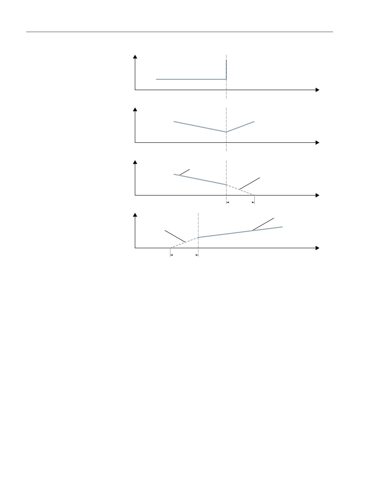
The function lowers the path velocity in continuou-path mode until the non-tangential block
transition can be traversed in one interpolation cycle while respecting the deceleration limit and
taking an overload factor into account.
With the reduced velocity, axial jumps in velocity are produced with a non-tangential contour at
the block transition. These jumps in velocity are also performed by the coupled motion
synchronized axes. The jump in velocity prevents the path velocity dropping to zero. This jump
is performed if the axial velocity was reduced with the axial acceleration to a velocity from which
the new setpoint can be reached with the jump. The magnitude of the setpoint jump can be
limited using an overload factor. Because the magnitude of the jump is axial, the minimum jump
of the path axes which are active during the block change is considered during block transition.
Basic functions
Function Manual, 10/2020, 6FC5397-2GP40-0BA1
447
Continuous-path mode, exact stop, LookAhead
6.3 Continuous-path mode
\
%ORFN FKDQJH
[
3DWK YHORFLW\
%ORFN FKDQJH
W
9HORFLW\ RI ; D[LV
$[LDO
*UDGLHQW D[
YHORFLW\ MXPS
*UDGLHQW I[ D[ I[ !
,32 F\FOH
W
$[LDO
9HORFLW\ RI < D[LV
*UDGLHQW D[
YHORFLW\ MXPS
*UDGLHQW I\ D\
I\ ! I[ !
I 2YHUORDG IDFWRU
,32 F\FOH
W
Figure 6-3
Axial velocity change on block transition
With a practically tangential block transition, the path velocity is not reduced if the permissible
axial accelerations are not exceeded. This means that very small bends in the contour (e.g. 0.5°)
are overtraveled directly.
Overload factor
The overload factor restricts step changes in the machine axis velocity at block ends. To ensure
that the velocity jump does not exceed the maximum load on the axis, the jump is derived from
the acceleration of the axis.
The overload factor indicates the extent by which the acceleration of the machine axis
(MD32300 $MA_MAX_AX_ACCEL) may be exceeded for an IPO-cycle.
The velocity jump results as follows:
Velocity jump = axis acceleration * (overload factor-1) * interpolator cycle.
The overload factor is saved in the machine data:
MD32310 $MA_MAX_ACCEL_OVL_FACTOR (overload factor for axial velocity jumps)
Factor 1.0 means that only tangential transitions with finite velocity can be traversed. For all
other transitions, the velocity is reduced to zero by changing the setpoint. This behavior is
Basic functions
448
Function Manual, 10/2020, 6FC5397-2GP40-0BA1
Continuous-path mode, exact stop, LookAhead
6.3 Continuous-path mode
equivalent to the function "Exact stop with interpolator end". This is undesirable for continuous-
path mode, so the factor must be set to greater than 1.0.
Note
For startup and installation, please note that the factor must be reduced if the machine is likely
to be subject to vibrations during angular block transitions and rounding is not to be used.
By setting the following machine data, the block transitions are rounded independent of the set
overload factor with G641/G642:
MD20490 $MC_IGNORE_OVL_FACTOR_FOR_ADIS
Activation/deactivation
Continuous-path mode with a reduction in speed according to the overload factor can be
activated in any NC part program block by the modal command G64.
Selecting the exact stop which works on a block-by-block basis enables rounding to be
interrupted (G9).
Continuous-path mode G64 can be deactivated by selecting:
• Modal exact stop G60
• Rounding G641, G642, G643, G644 or G645
Implicit continuous-path mode
If it is not possible to insert rounding blocks in continuous-path mode with rounding G641 due
to the very short block path lengths (e.g. zero-clocked blocks), the mode is switched over to
continuous-path mode G64.
6.3.3
Rounding
Function
The "Rounding" function adds intermediate blocks (positioning blocks) along a programmed
contour (path axes) at non-continuous (angular) block transitions so that the resulting new
block transition is continuous (tangential).
Synchronized axes
The rounding considers not only the geometry axes but also all synchronous axes. Although a
continuous block transition cannot be created for both axis types concurrently for the parallel
travel of path and synchronous axes. In this case, to favor path axes that always travel exactly,
only an approximately continuous block transition is created for synchronous axes.
Basic functions
Function Manual, 10/2020, 6FC5397-2GP40-0BA1
449
Continuous-path mode, exact stop, LookAhead
6.3 Continuous-path mode
Rounding for G64
Rounding is performed even when to observe the dynamic-response limits at the block
transition, a speed is required that for G64 exceeds the permitted speed at the block transition
(see Section "Velocity reduction according to overload factor (Page 447)" "Overload factor").
Impact on synchronization conditions
The use of rounding shortens the programmed blocks between which the rounding block(s) are
added. The programmed block boundary disappears and are then no longer available as
criterion for any synchronization conditions (e.g. auxiliary function output parallel to motion,
stop at block end).
Note
We recommend that when the "Rounding" function is used, synchronization conditions apply to
the end of the block before the rounding location rather than the end of the inserted rounding
block. The following block would then not be started and with a stop at the block end, the
contour of the following block can still be changed manually.
Exceptions
In the following cases, no rounding occurs at the block transition, for example, between the N10
blocks after N20, i.e. no rounding block is added:
Implicit stopping of the traversing motion
Possible causes:
• Auxiliary function output active before the traversing motion for N20
• N20 does not contain any traversing motion for path axes
• In N20, an axis that was previously a positioning axis traverses as a path axis for the first time
• In N20, an axis that was previously a path axis traverses as a positioning axis for the first time
• Geometry axes traverse in N10 but not in N20
• Geometry axes traverse in N20 but not in N10
• Activation of thread-cutting G33 in N20
• Change from BRISK and SOFT
• Transformation-relevant axes are not completely assigned to the path motion (e.g. for
oscillation axes, positioning axes).
Basic functions
450
Function Manual, 10/2020, 6FC5397-2GP40-0BA1
Continuous-path mode, exact stop, LookAhead
6.3 Continuous-path mode
The insertion of the rounding block would slow part program machining
overproportionally
Possible causes:
• A program or program section consists of a number of very short traversal blocks (≈ 1
interpolator cycle / traversal block; because each traversal block requires at least one
interpolator cycle, the inserted intermediate block would almost double the machining time)
• G64 (path control operation without rounding) without speed reduction active for block
change
• The parameterized overload factor (MD32310 $MA_MAX_ACCEL_OVL_FACTOR) permits the
traversal of the programmed contour without the path speed needing to be reduced. See
also: MD20490 $MC_IGNORE_OVL_FACTOR_FOR_ADIS
Path parameters inhibit the rounding
Possible causes:
• G641 (path control operation with rounding in accordance with the path criterion) is active
but rapid traverse is active (G0) AND ADISPOS == 0 (rounding separation for G0)
• G641 (path control operation with rounding in accordance with the path criterion) is active
but rapid traverse is not active AND ADIS == 0 (rounding separation for path functions G1,
G2, G3, ...)
• G642 or G643 (path control operation with rounding while observing defined tolerances) is
active but all tolerances == zero
N10 or N20 does not contain traversing motion (zero block).
Normally no zero blocks are created. Exceptions:
• Active synchronous action
• Program jumps
Impact on synchronization conditions
The programmed blocks between which the rounding contour is added are shortened during
rounding. The original programmed block boundary disappears and is then no longer available
for any synchronization conditions (e.g. auxiliary function output parallel to motion, stop at
block end).
Note
We recommend that when the "Rounding" function is used, synchronization conditions apply to
the end of the block before the rounding location rather than the end of the inserted rounding
block. The following block would then not be started and with a stop at the block end, the
contour of the following block can still be changed.
Basic functions
Function Manual, 10/2020, 6FC5397-2GP40-0BA1
451
Continuous-path mode, exact stop, LookAhead
6.3 Continuous-path mode
6.3.3.1
Rounding according to a path criterion (G641)
Function
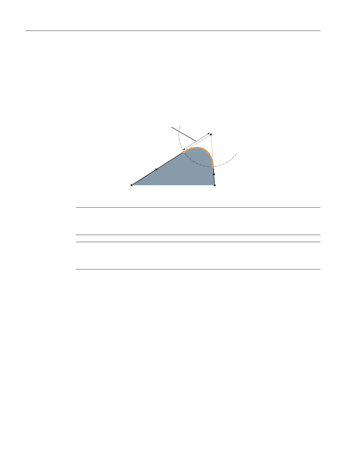
In continuous-path mode with rounding according to a path criterion, the size of the rounding
area is influenced by the path criteria ADIS and ADISPOS.
The path criteria ADIS and ADISPOS describe the maximum distances which a rounding block can
occupy before and after a block.
3DWK FULWHULRQ
$',6
3URJUDPPHG
$',6326
LQWHUPHGLDWH SRLQW LQ EORFN
3URJUDPPHG LQSXW EORFN
3URJUDPPHG RXWSXW
EORFN
Note
Acute angles produce rounding curves with a large degree of curvature and therefore cause a
corresponding reduction in velocity.
Note
ADISPOS is programmed in the same way as ADIS, but must be used specifically for movements
in rapid traverse mode G0.
Scope of the path criterion
• ADIS or ADISPOS must be programmed. If the default is "zero", G641 behaves like G64.
• If only one of the blocks involved is rapid traverse G0, the smaller rounding distance applies.
Basic functions
452
Function Manual, 10/2020, 6FC5397-2GP40-0BA1
Continuous-path mode, exact stop, LookAhead
6.3 Continuous-path mode
•
If a very small value is used for ADIS, the controller must make sure that every interpolated
block, even an intermediate rounding block, contains at least one interpolation point. The
maximum path velocity is thereby limited to ADIS / interpolator cycle.
•
Irrespective of ADIS and ADISPOS, the rounding area is limited by the block length.
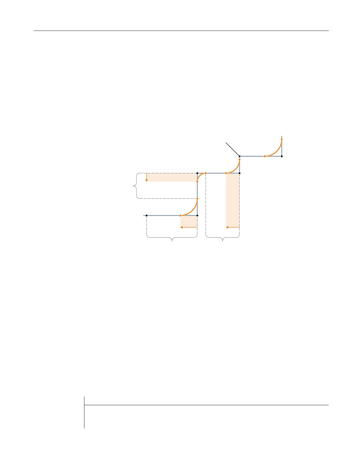
In blocks with short distances (distance < 4* ADIS and < 4 * ADISPOS respectively), the
rounding distance is reduced so that a traversable part of the original block is retained. The
remaining length depends on the axis path and is approximately 60% of the distance still to
be traversed in the block. ADIS or ADISPOS is therefore reduced to the remaining 40% of the
distance to be traversed. This algorithm prevents a rounding block being inserted for a very
small change in contour. In this case, switchover to continuous-path mode G64 is automatic
until rounding blocks can be inserted again.
1R VPRRWKLQJ
1
1
1
$',6
5HPDLQLQJ SDWK
1
1
6WDUW RI EORFN 1
1
$',6
$',6
5HPDLQLQJ SDWK
5HPDLQLQJ SDWK
1
1
Figure 6-4
Path with limitation of ADIS
Activation/deactivation
Continuous-path mode with rounding based on a path criterion can be activated in any NC part
program block by the modal command G641. Before or on selection, the path criteria ADIS/
ADISPOS must be specified.
Selecting the exact stop which works on a block-by-block basis enables rounding to be
interrupted (G9).
Continuous-path mode with rounding based on a path criterion (G641) can be deactivated by
selecting:
• Modal exact stop (G60)
• Continuous-path mode G64, G642, G643, G644 or G645
Program example
Program code
Comment
N1 G641 Y50 F10 ADIS=0.5
; Continuous-path mode with rounding based on a path
criterion (rounding clearance: 0.5 mm)
N2 X50
Basic functions
Function Manual, 10/2020, 6FC5397-2GP40-0BA1
453

Continuous-path mode, exact stop, LookAhead
6.3 Continuous-path mode
Program code
Comment
N3 X50.7
N4 Y50.7
N5 Y51.4
N6 Y51.0
N7 X52.1
6.3.3.2
Rounding in compliance with defined tolerances (G642/G643)
Function
In continuous-path mode involving rounding in compliance with defined tolerances, the
rounding normally takes place while adhering to the maximum permissible path deviation.
Instead of these axis-specific tolerances, the maintenance of the maximum contour deviation
(contour tolerance) or the maximum angular deviation of the tool orientation (orientation
tolerance) can be configured.
Activation
Continuous-path mode with rounding in compliance with defined tolerances can be activated in
any NC part program block by the modal command G642 or G643.
Selecting the exact stop which works on a block-by-block basis enables rounding to be
interrupted (G9).
Continuous-path mode with rounding in compliance with defined tolerances (G642/G643) can
be deactivated by selecting:
• Modal exact stop (G60)
• Continuous-path mode G64, G641, G644 or G645
Differences between G642 - G643
With regard to their rounding behavior, commands G642 and G643 differ as follows:
G642
G643
With G642, the rounding path is determined on the
In the case of G643, each axis may have a different
basis of the shortest distance for rounding all axes.
rounding path. The rounding travels are taken into
This value is taken into account when generating a
account axis-specifically and block-internally (⇒ no
rounding block.
separate rounding block).
With G642, the rounding area results from the
Very different specifications for the contour toler-
smallest tolerance setting.
ance and the tolerance of the tool orientation can
only have effect with G643.
Parameterization
Maximum path deviation
The maximum path deviation permitted with G642/G643 is set for each axis in the machine data:
Basic functions
454
Function Manual, 10/2020, 6FC5397-2GP40-0BA1

Continuous-path mode, exact stop, LookAhead
6.3 Continuous-path mode
MD33100 $MA_COMPRESS_POS_TOL
Contour tolerance and orientation tolerance
The contour tolerance and orientation tolerance are set in the channel-specific setting data:
SD42465 $SC_SMOOTH_CONTUR_TOL (maximum contour deviation)
SD42466 $SC_SMOOTH_ORI_TOL (maximum angular deviation of the tool orientation)
The settings data can be programmed in the NC program and can in this way be specified
differently for each block transition.
Note
The setting data SD42466 $SC_SMOOTH_ORI_TOL is effective only in active orientation
transformation.
Rounding behavior
Rounding behavior with G642 and G643 is configured via the machine data:
MD20480 $MC_SMOOTHING_MODE (rounding behavior with G64x)
The units positions (E) define the behavior for G643, the tens positions (Z) the behavior for G642:
Value E or Z
Meaning
0
All axes:
Rounding by maintaining the maximum permitted path deviation:
MD33100 $MA_COMPRESS_POS_TOL
1
Geometry axes:
Rounding by maintaining the contour tolerance:
SD42465 $SC_SMOOTH_CONTUR_TOL
Remaining axes:
Rounding by maintaining the maximum permitted path deviation:
MD33100 $MA_COMPRESS_POS_TOL
2
Geometry axes:
Rounding by maintaining the orientation tolerance:
SD42466 $SC_SMOOTH_ORI_TOL
Remaining axes:
Rounding by maintaining the maximum permitted path deviation:
MD33100 $MA_COMPRESS_POS_TOL
Basic functions
Function Manual, 10/2020, 6FC5397-2GP40-0BA1
455

Continuous-path mode, exact stop, LookAhead
6.3 Continuous-path mode
Value E or Z
Meaning
3
Geometry axes:
Rounding by maintaining the contour tolerance and the orientation tolerance:
SD42465 $SC_SMOOTH_CONTUR_TOL
SD42466 $SC_SMOOTH_ORI_TOL
Remaining axes:
Rounding by maintaining the maximum permitted path deviation:
MD33100 $MA_COMPRESS_POS_TOL
4
All axes:
The rounding length programmed with ADIS or with ADISPOS is used (as in case of
G641).
Any axis-specific tolerance or contour and orientation tolerance specifications are ig-
nored.
Profile for limit velocity
The use of a velocity profile for rounding in compliance with defined tolerances is controlled via
the hundreds position in MD20480:
Value
Meaning
< 100:
A profile of the limit velocity is calculated within the rounding area, based on the defined
maximum values for acceleration and jerk on the participating axes or path.
This can lead to an increase in the path velocity in the rounding area and therefore to the
acceleration of the participating axes.
≥100:
A profile of the limit velocity is not calculated for rounding blocks with G641/G642. A
constant velocity limit is specified instead.
This prevents the participating axes being accelerated into the rounding area during
rounding with G641/G642. However, in certain cases, this setting can cause the rounding
blocks to be traversed too slowly, especially in large rounding areas.
1xx:
No velocity profile for G641
2xx:
No velocity profile for G642
Note
MD28530 $MC_MM_PATH_VELO_SEGMENTS (number of memory elements for limiting the
path velocity)
Supplementary conditions
Restriction for protection zones with active radius compensation and tool orientation:
Although tool radius compensation is applied for a tool orientation, which is not perpendicular
to one of the three datum planes of the basic coordinate system, the protection zones are not
rotated onto the corresponding plane.
For G643 the following must apply:
MD28530 $MC_MM_PATH_VELO_SEGMENTS > 0 (number of memory elements for limiting the
path velocity)
If this condition is met, then it must be applicable for all axes:
Basic functions
456
Function Manual, 10/2020, 6FC5397-2GP40-0BA1

Continuous-path mode, exact stop, LookAhead
6.3 Continuous-path mode
MD35240 $MC_ACCEL_TYPE_DRIVE = FALSE (acceleration characteristic DRIVE for axes on/off)
6.3.3.3
Rounding with maximum possible axial dynamic response (G644)
Function
Maximizing the dynamic response of the axes is key to this type of continuous-path mode with
smoothing.
Note
Smoothing with G644 is only possible under the following conditions:
• All of the participating axes contain only one linear motion in the two blocks under
consideration.
• A kinematic transformation is not active.
If a participating axis contains a polynomial (polynomial programmed, spline active, compressor
active) or a kinematics transformation is active (PTP travel temporarily deactivates a kinematics
transformation), the block transition is smoothed with G642.
Activation
Continuous-path mode with smoothing with the maximum possible axial dynamic response can
be activated in any NC part program block by the modal command G644.
Selecting the exact stop which works on a block-by-block basis enables smoothing to be
interrupted (G9).
Continuous-path mode with smoothing with the maximum possible axial dynamic response
(G644) can be deactivated by selecting:
• Modal exact stop (G60)
• Continuous-path mode G64, G641, G642, G643 or G645
Parameter assignment
Smoothing behavior with G644 is configured via the thousands and tens of thousands places in
the machine data:
MD20480 $MC_SMOOTHING_MODE (smoothing behavior with G64x)
Value
Meaning
Thousand's place:
0xxx:
When smoothing with G644, the maximum deviations for each axis specified by the following
machine data are respected:
MD33100 $MA_COMPRESS_POS_TOL
If the dynamics of the axis permit, then any specified tolerance is not utilized.
Basic functions
Function Manual, 10/2020, 6FC5397-2GP40-0BA1
457

Continuous-path mode, exact stop, LookAhead
6.3 Continuous-path mode
Value
Meaning
1xxx:
Specification of the maximum smoothing path by programming ADIS=...
or ADISPOS=... (as for G641).
2xxx:
Input the maximum possible frequencies of each axis in the smoothing area using the ma-
chine data:
MD32440 $MA_LOOKAH_FREQUENCY (smoothing frequency for LookAhead)
The smoothing area is defined so that no frequencies in excess of the specified maximum can
occur while the smoothing motion is in progress.
3xxx:
Any axis that has a velocity jump at a corner traverses around the corner with the maximum
possible dynamic response (maximum acceleration and maximum jerk).
SOFT:
If SOFT is active, the maximum acceleration and the maximum jerk of each axis are main-
tained.
BRISK:
If BRISK is active, only the maximum acceleration and not the maximum jerk of each axis is
maintained.
With this setting, neither the maximum deviations nor the smoothing distance are checked.
The resulting deviations or smoothing distances are determined exclusively by the dynamic
limits of the respective axis and the current path velocity.
4xxx:
As in case of 0xxx, the maximum deviations of each axis specified with the following machine
data are used:
MD33100 $MA_COMPRESS_POS_TOL
Contrary to 0xxx, the specified tolerance is also utilized, if possible. Therefore, the axis does
not attain its maximum possible dynamics.
5xxx:
As in case of 1xxx, the maximum possible smoothing path is specified through programming
of ADIS=... or ADISPOS=... respectively.
Contrary to 1xxx, the specified smoothing path is also utilized, if possible. Therefore, the axes
involved do not attain their maximum possible dynamics.
Ten thousands digit
0xxxx
The velocity profiles of the axes in the smoothing area are determined without jerk limiting
for BRISK and with jerk limiting for SOFT.
1xxxx
The velocity profiles of the axes in the smoothing area are always determined with jerk
limiting, regardless of whether BRISK or SOFT is active.
When specifying the maximum axial deviations (MD33100 $MA_COMPRESS_POS_TOL) or the
maximum smoothing distance (ADIS / ADISPOS) the available smoothing path is normally not
used, if permitted by the dynamic response of the axes involved. Through this, the length of the
smoothing path depends on the active path feedrate. In case of lower path speeds, one gets
lower deviations from the programmed contours. However, it can be set that in these cases the
specified maximum axial deviation or the specified smoothing distance is utilized, if possible. In
this case the deviations depend on the programmed contour independent of the programmed
path feedrate.
Note
Apart from the ones mentioned, the following limitation can also become active additionally:
The smoothing distance cannot exceed half the length of the original participating blocks.
Basic functions
458
Function Manual, 10/2020, 6FC5397-2GP40-0BA1
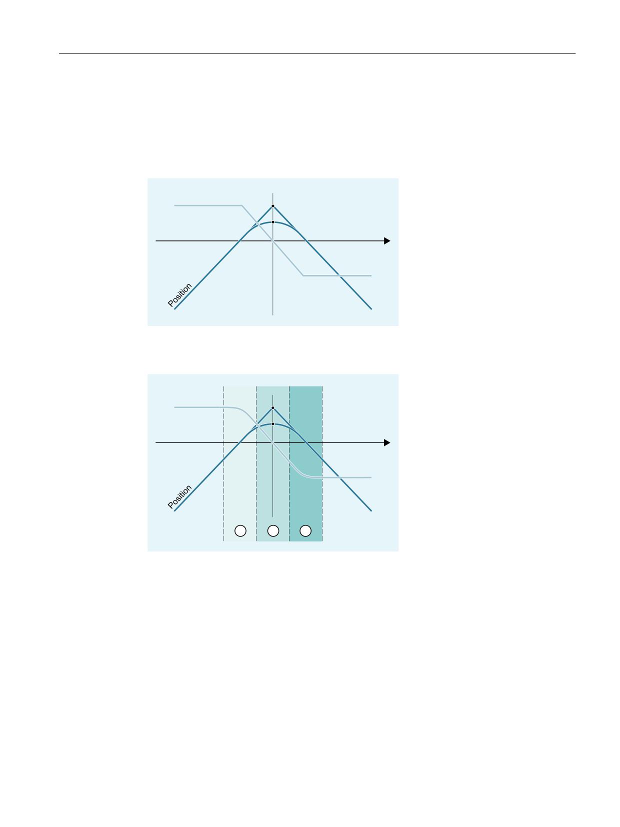
Continuous-path mode, exact stop, LookAhead
6.3 Continuous-path mode
Jerk limitation
The smoothing of the velocity jump on each axis and thus the shape of the smoothing path
depends on whether an interpolation is performed with or without jerk limitation.
Without jerk limitation the acceleration of each axis reaches its maximum value in the entire
smoothing area:
9HORFLW\
7LPH
With jerk limitation, the jerk of each axis is limited to its maximum value within the smoothing
area. The smoothing motion thus generally consists of 3 phases(① ... ③):
9HORFLW\
7LPH
① During phase 1, each axis builds up its maximum acceleration. The jerk is constant and equal to the
maximum possible jerk on the respective axis.
② During phase 2, the maximum permissible acceleration is applied.
③ During phase 3, which is the last phase, the acceleration of each axis is reduced back to zero with
the maximum permissible jerk.
6.3.3.4
Rounding of tangential block transitions (G645)
Function
In continuous-path mode with rounding, rounding blocks are also only generated on tangential
block transitions if the curvature of the original contour exhibits a jump in at least one axis.
Basic functions
Function Manual, 10/2020, 6FC5397-2GP40-0BA1
459
Continuous-path mode, exact stop, LookAhead
6.3 Continuous-path mode
The rounding motion is defined here so that the acceleration of all axes involved remains smooth
(no jumps) and the parameterized maximum deviations from the original contour
(MD33120 $MA_PATH_TRANS_POS_TOL) are not exceeded.
In the case of angular, non-tangential block transitions, the rounding behavior is the same as
with G642 (see Section "Rounding in compliance with defined tolerances (G642/G643)
(Page 454)").
Activation/deactivation
Continuous-path mode with rounding of tangential block transitions can be activated in any NC
part program block by the modal command G645.
Selecting the exact stop which works on a block-by-block basis enables rounding to be
interrupted (G9).
Continuous-path mode with rounding of tangential block transitions (G645) can be deactivated
by selecting:
• Modal exact stop (G60)
• Continuous-path mode G64, G641, G642, G643 or G644
Comparison between G642 and G645
When rounding with G642, the only block transitions rounded are those which form a corner,
i.e. the velocity of at least one axis jumps. However, if a block transition is tangential, but there
is a jump in the curvature, no rounding block is inserted with G642. If this block transition is
traversed with finite velocity, the axes experience some degree of jump in acceleration which
(with the jerk limit activated!) may not exceed the parameterized limit (MD32432
$MA_PATH_TRANS_JERK_LIM). Depending on the level of the limit, the path velocity at the block
transition may be greatly reduced as a result. This constraint is avoided by using G645 because
the rounding motion is defined here in such a way that no jumps occur in acceleration.
Parameterization
The following machine data indicates the maximum permissible path deviation for each axis
during rounding with G645:
MD33120 $MA_PATH_TRANS_POS_TOL
This value is only of relevance to tangential block transitions with variable acceleration. When
angular, non-tangential block transitions are rounded, (as with G642) the tolerance from
MD33100 $MA_COMPRESS_POS_TOL becomes effective.
See also
Free-form surface mode: Basic functions (Page 486)
Basic functions
460
Function Manual, 10/2020, 6FC5397-2GP40-0BA1
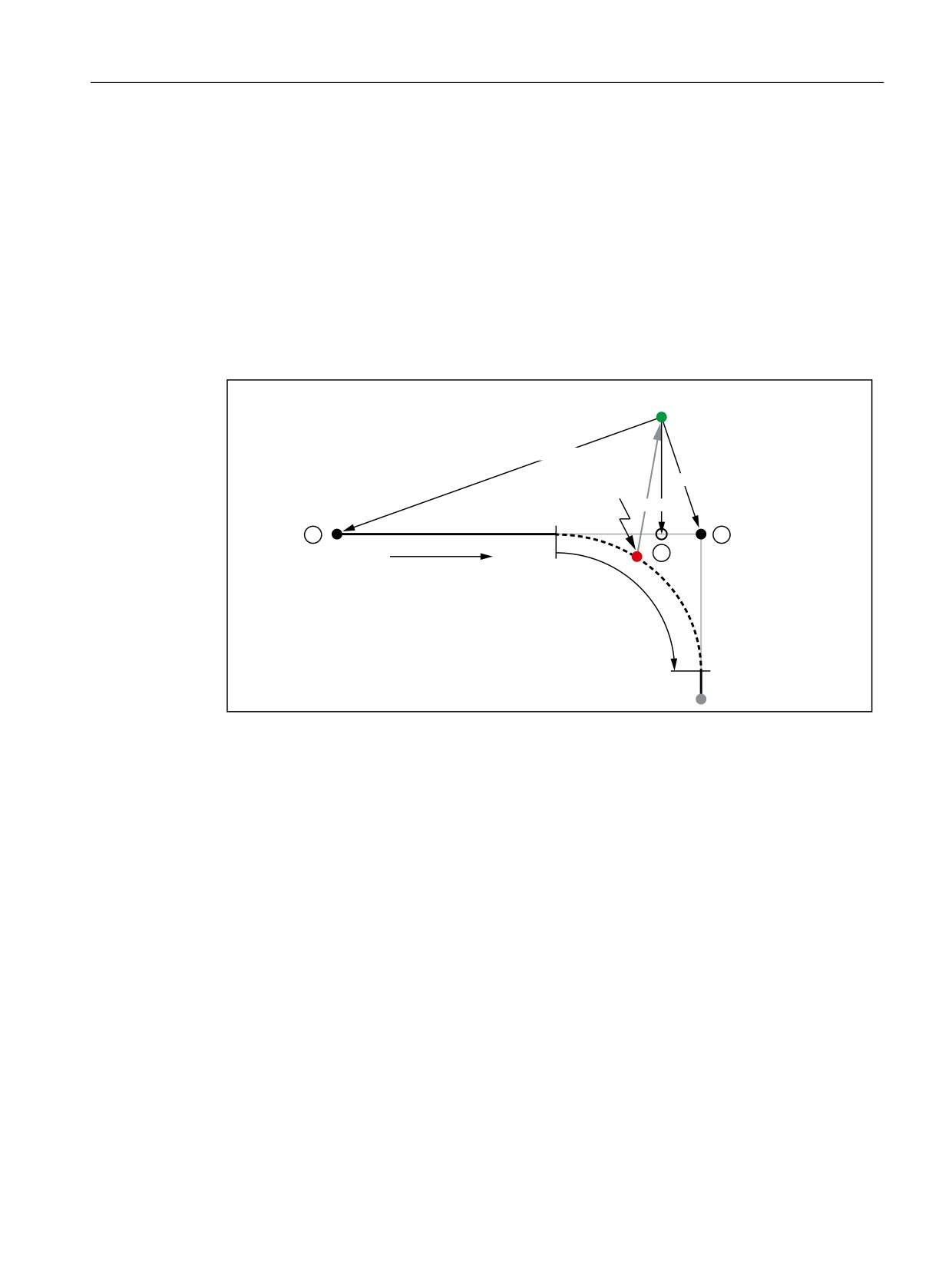
Continuous-path mode, exact stop, LookAhead
6.3 Continuous-path mode
6.3.3.5
Rounding and repositioning (REPOS)
If the machining in the area of the rounding contour is interrupted, a REPOS operation cannot
be used to position again directly on the rounding contour. In this case, positioning can be made
only on the programmed contour.
Example
Programmed: Two traversing blocks N10 and N20 with programmed rounding G641.
The traversing motion is interrupted in the rounding area. The axes, e.g. manually, are then
traversed to the REPOS start point. Depending on the selected REPOS mode, the repositioning
on the contour is made at the points ①, ② or ③.
5(326 VWDUWLQJ SRLQW
50%%/
50,%/
50(%/
%UHDN SRLQW
501%/
1
7UDYHUVLQJ
GLUHFWLRQ
6PRRWKLQJ VHW
1
RMBBL
Repositioning at the start of the interrupted traversal block
RMIBL
Repositioning at the interruption location
RMEBL
Repositioning at the end of the interrupted traversal block
RMNBL
Repositioning at the next contour point
①
Block start N10
②
To the REPOS start point of the next contour point
③
Block end N10 / block start N20
Basic functions
Function Manual, 10/2020, 6FC5397-2GP40-0BA1
461
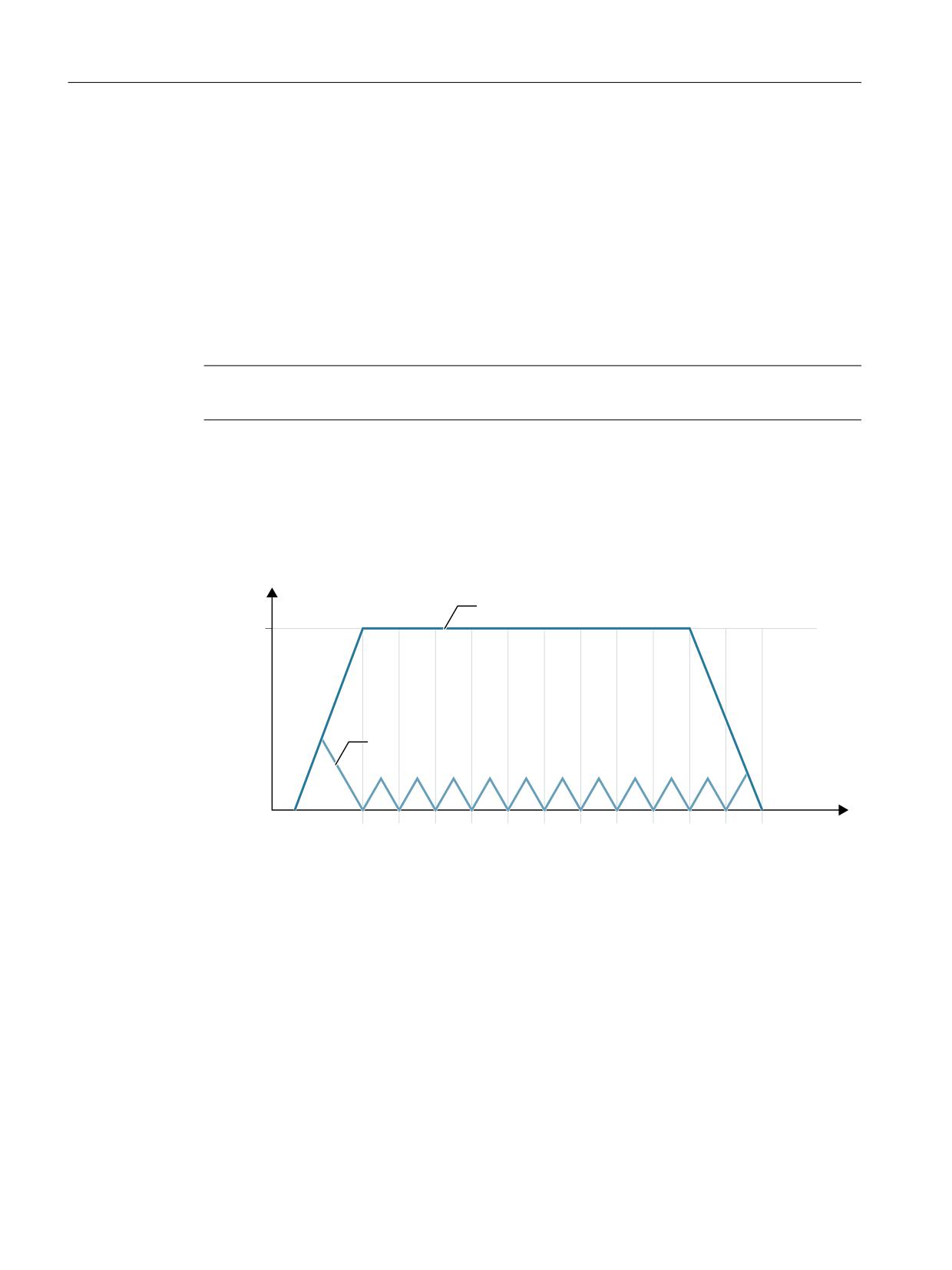
Continuous-path mode, exact stop, LookAhead
6.3 Continuous-path mode
6.3.4
LookAhead
6.3.4.1
Standard functionality
Function
LookAhead is a function which is active in continuous-path mode (G64, G64x) and determines
a foreseeable velocity control for multiple NC part program blocks over and beyond the current
block.
Note
LookAhead is only available for path axes, not for spindles and positioning axes.
If a part program contains consecutive blocks with very small paths, only one velocity is reached
per block without LookAhead, enabling deceleration of the axes at the end of the block while
maintaining acceleration limits. This means that the programmed velocity is not reached at all.
With LookAhead, however, it is possible to implement the acceleration and deceleration phase
over multiple blocks with approximately tangential block transitions, thereby achieving a higher
feedrate with shorter distances.
)HHGUDWH
*
3UHGLFWLYH YHORFLW\ FRQWURO
SURJUDPPHG
)
*
&RQV
WDQW YH
ORFLW\ SKDVH
FDQQR
W EH
UHDFKHG
1
1
1
1
1
1
1
1
1
1
1
1
%ORFN SDWK
Figure 6-5
Velocity control with short distances and exact stop G60 or continuous-path mode G64 with
LookAhead
Deceleration to velocity limits is possible with LookAhead such that violation of the acceleration
and velocity limit is prevented.
LookAhead takes plannable velocity limits into consideration such as:
• Exact stop at block end
• Velocity limit in the block
• Acceleration limit in the block
• Velocity limit on block transition
• Synchronization with block change at block transition.
Basic functions
462
Function Manual, 10/2020, 6FC5397-2GP40-0BA1
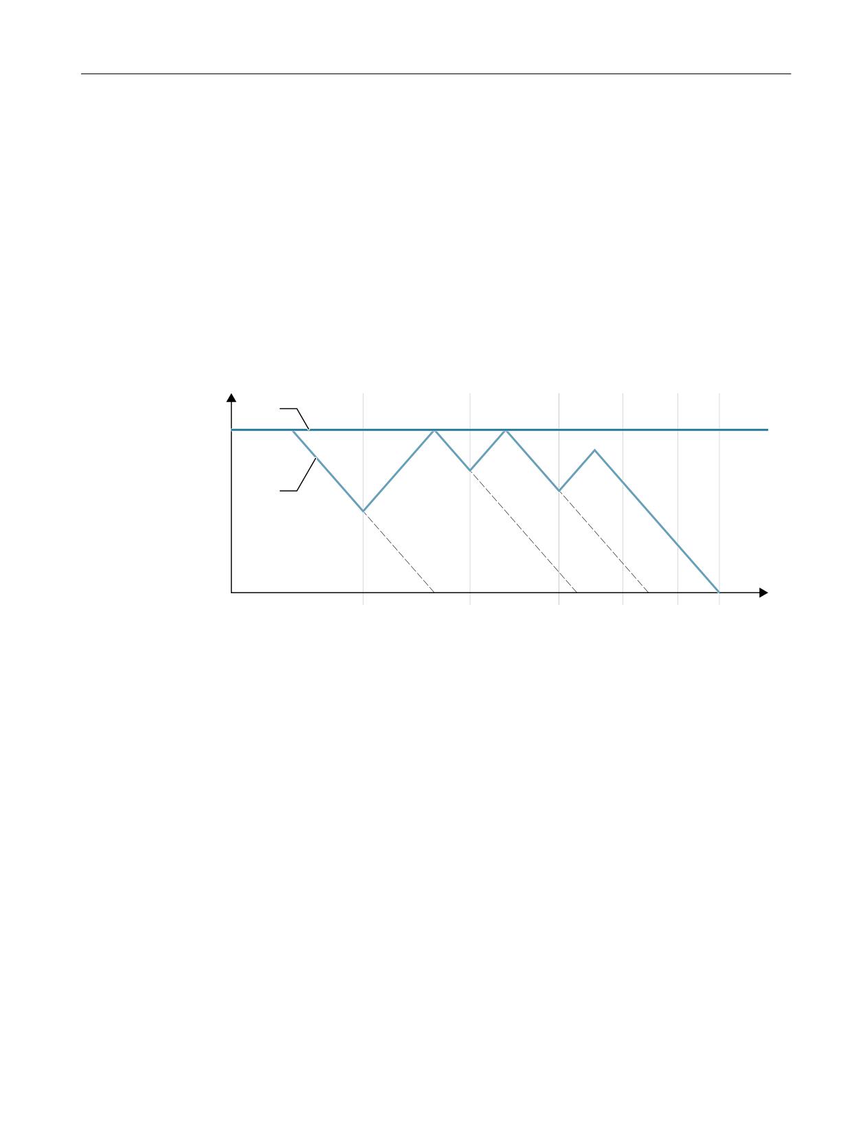
Continuous-path mode, exact stop, LookAhead
6.3 Continuous-path mode
Mode of operation
LookAhead carries out a block-specific analysis of velocity limits and specifies the required brake
ramp profile based on this information. LookAhead is adapted automatically to block length,
braking capacity and permissible path velocity.
For safety reasons, the velocity at the end of the last prepared block must initially be assumed
to be zero because the next block might be very small or be an exact-stop block, and the axes
must have been stopped by the end of the block.
With a series of blocks with high set velocity and very short paths, the speed can be increased
in each block depending on the velocity value currently calculated by the LookAhead function
in order to achieve the required set velocity. After this it can be reduced so that the velocity at
the end of the last block considered by the LookAhead function can be zero. This results in a
serrated velocity profile (see the following fig.) which can be avoided by reducing the set velocity
or increasing the number of blocks considered by the LookAhead function.
Y
9VHWSRLQW
9DFW
1
1
1
1
1
1
W
Figure 6-6
Example for modal velocity control (number of blocks considered by the LookAhead function
= 2)
Activation/deactivation
LookAhead is activated by selecting continuous-path mode G64, G641, G642, G643, G644 or
G645.
Selecting the exact stop which works on a non-modal basis enables rounding to be interrupted
(G09).
LookAhead is deactivated by selecting the modal exact stop (G60).
Parameterization
Number of blocks
To achieve reliable axis traversal in continuous-path mode, the feedrate must be adapted over
several blocks. The number of blocks considered by the LookAhead function is calculated
automatically and can, if required, be limited by a machine data. The default setting is "1", which
means that LookAhead only considers the following block for velocity control.
Because LookAhead is especially important for short blocks (relative to the deceleration path),
the number of blocks required is of interest for LookAhead braking. It is sufficient to consider the
Basic functions
Function Manual, 10/2020, 6FC5397-2GP40-0BA1
463
Continuous-path mode, exact stop, LookAhead
6.3 Continuous-path mode
path length to be equal to the deceleration path that is required to brake from maximum velocity
to standstill.
For a machine with a low axial acceleration of a = 1 m/s2 and a high feedrate of vpath = 10 m/min,
the following number of nLookAhead blocks are allocated to the controller where it has an attainable
block cycle time of TB = 10 ms:
nLookAhead = Deceleration path/Block length = ( vpath2 / (2a)) / (vpath * TB) = 9
Considering these conditions, it is advisable to adapt the feedrate over 10 blocks. The number
of blocks entered for the LookAhead function forecast does not change the LookAhead
algorithm and memory requirement.
Since the machining velocity is very often set to a lower value than the maximum velocity in a
program, more blocks than are required would be predicted, overloading the processor
unnecessarily. For this reason, the required number of blocks is derived from the velocity which
is calculated from the following multiplication:
• Programmed velocity * MD12100 $MN_OVR_FACTOR_LIMIT_BIN
(when using a binary-coded feedrate override switch)
• Programmed velocity * MD12030 $MN_OVR_FACTOR_FEEDRATE[30]
(when using a Gray-coded feedrate override switch)
The value for MD12100 or the 31st override value for MD12030 defines the dynamic response
reserves which the velocity control provides for when the path feedrate is overshot.
Note
The 31st override value for MD12030 should correspond to the highest override factor which is
actually used.
Note
The number of blocks considered by the LookAhead function is limited by the possible number
of NC blocks in the IPO buffer.
Velocity profiles
In addition to the fixed, plannable velocity limitations, LookAhead can also take account of the
programmed velocity. This makes it possible to achieve a lower velocity by applying LookAhead
beyond the current block.
• Determination of the following block velocity
One possible velocity profile contains the determination of the following block velocity.
Using information from the current and the following NC block, a velocity profile is calculated
from which, in turn, the required velocity reduction for the current override is derived.
The calculated maximum value of the velocity profile is limited by the maximum path velocity.
With this function it is possible to initiate a speed reduction in the current block taking
override into account such that the lower velocity of the following block can be achieved. If
the reduction in velocity takes longer than the travel time of the current block, the velocity
is further reduced in the following block. Velocity control is only ever considered for the
following block.
The function is activated via the machine data:
MD20400 $MC_LOOKAH_USE_VELO_NEXT_BLOCK
Basic functions
464
Function Manual, 10/2020, 6FC5397-2GP40-0BA1

Continuous-path mode, exact stop, LookAhead
6.3 Continuous-path mode
Value
Meaning
TRUE
Function active
FALSE
Function not active
Basic functions
Function Manual, 10/2020, 6FC5397-2GP40-0BA1
465
Continuous-path mode, exact stop, LookAhead
6.3 Continuous-path mode
• Definition of override points
If the velocity profile of the following block velocity is not sufficient because, for example,
very high override values (e.g. 200%) are used or a constant cutting rate G96/G961 is active,
with the result that the velocity must be further reduced in the following block, LookAhead
provides a way of reducing the programmed velocity over several NC blocks.
By defining override points, LookAhead calculates a limiting velocity profile for each value.
The required velocity reductions for the current override are derived from these profiles.
The calculated maximum value of the velocity profile is limited by the maximum path velocity.
The upper point should cover the velocity range that will be reached by the maximum value
set in the machine data:
MD12030 $MN_OVR_FACTOR_FEEDRATE[n] (evaluation of the path feedrate override
switch)
It can also be reached via the value of the machine data:
MD12100 $MN_OVR_FACTOR_LIMIT_BIN (limit for binary-coded override switch)
In this way, a reduction of the velocity continuing into the block in which it is programmed
can be avoided.
If velocity reductions across block boundaries are required at a 100% override, a point should
be set in the lower override range as well.
The number of override points used per channel is specified in the machine data:
MD20430 $MC_LOOKAH_NUM_OVR_POINTS (number of override switch points for
LookAhead)
The associated points are stored in the machine data:
MD20440 $MC_LOOKAH_OVR_POINTS (override switch points for LookAhead)
Example:
Limiting velocity characteristics, whereby:
- Override = 50%, 100% or 150%
- Number of LookAhead blocks = 4
- MD20430 $MC_LOOKAH_NUM_OVR_POINTS = 2
- MD20440 $MC_LOOKAH_OVR_POINTS = 1.5, 0.5
Basic functions
466
Function Manual, 10/2020, 6FC5397-2GP40-0BA1
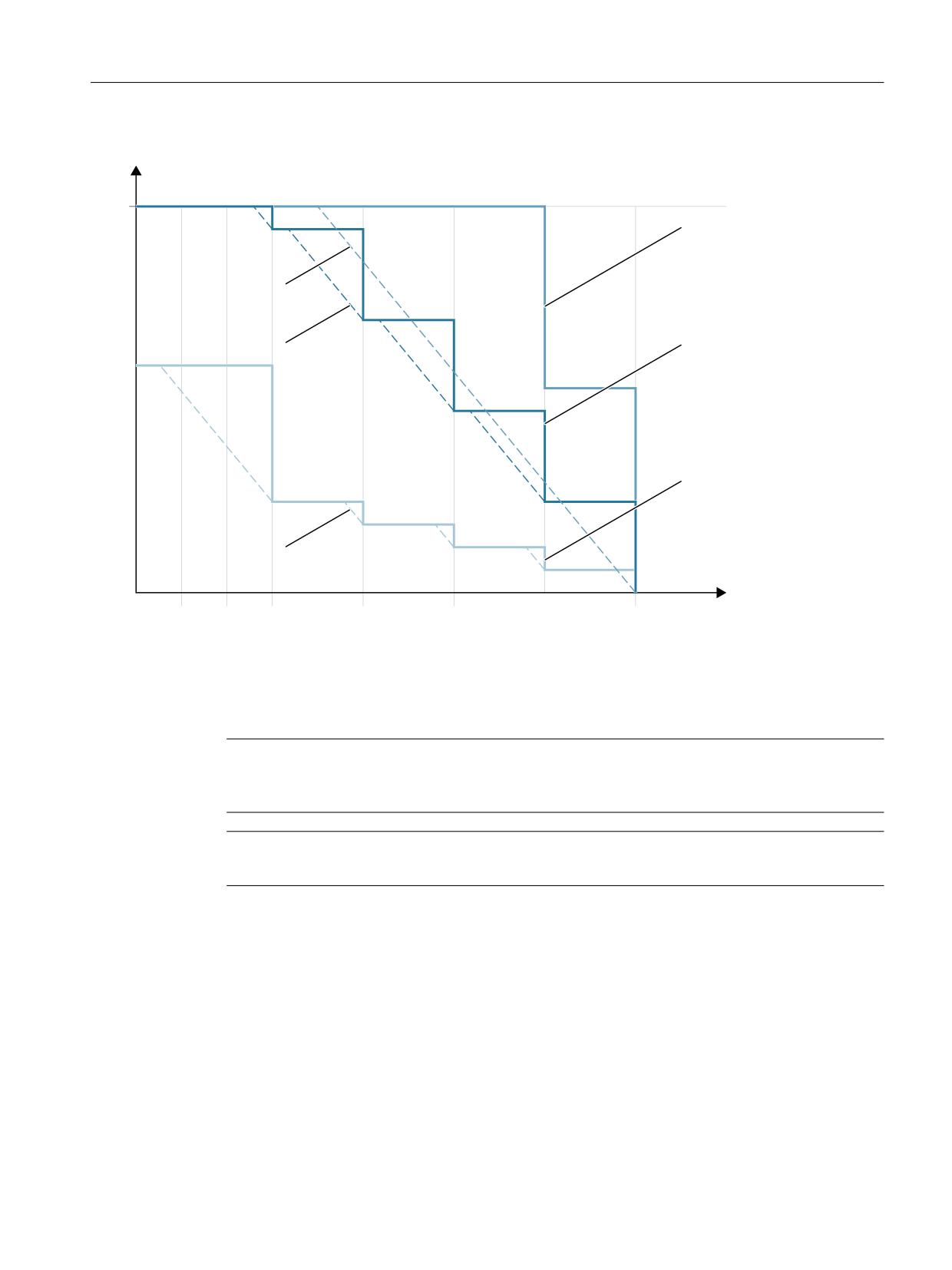
Continuous-path mode, exact stop, LookAhead
6.3 Continuous-path mode
- MD20400 $MC_LOOKAH_USE_VELO_NEXT_BLOCK = 1
Y
YtPD[
9HORFLW\ SURILOH
2YHUU
LGH
2YHUU
LGH
3URJUDPPHG VHWSRLQW
9HORFLW\ SURILOH
9HORFLW\ SURILOH
2YHUULGH
1
1
1
1
1
V
A combination of both procedures (determination of following block velocity and determination
of override points) can be used to calculate the velocity profiles and is generally advisable
because the preset machine data for these functions already takes the widest range of override-
dependent velocity limits into account.
Note
If neither of the procedures has been activated, the setpoint velocity is always applied in the
current block.
Note
Plannable velocity limits restrict override-specific velocity limits.
Relief factor with block cycle problems
Block cycle problems are encountered in cases where the traversing distances of the NC blocks
to be processed are so short that the LookAhead function has to reduce the machine velocity to
provide enough time for block processing. In this situation, constant braking and acceleration
of path motion may occur.
Velocity fluctuations of this type can be dampened by specifying a relief factor:
MD20450 $MC_LOOKAH_RELIEVE_BLOCK_CYCLE (relieving factor for the block cycle time)
Basic functions
Function Manual, 10/2020, 6FC5397-2GP40-0BA1
467
Continuous-path mode, exact stop, LookAhead
6.3 Continuous-path mode
Boundary conditions
Axis-specific feed stop/axis disable
Axis-specific feed stop and axis-specific axis disable are ignored by LookAhead.
If an axis is to be interpolated that should on the other hand be made stationary by axis-specific
feed stop or axis disable, LookAhead does not stop path motion before the block in question but
decelerates in the block itself.
If this response is not wanted, an axis-specific feed stop can be transferred to a channel via the
PLC to stop the path immediately (see also Function Manual Monitoring and Compensating,
Section Clamping monitoring).
6.3.4.2
Free-form surface mode: Extension function
Function
The "Free-form surface mode: Extension function" is an extension of the Look Ahead standard
functionality and is used to calculate the path velocity profile during free-form surface
machining (see also Section "Free-form surface mode: Basic functions (Page 486)").
Its use optimizes the continuous-path mode as follows:
• Symmetry between the acceleration and deceleration profiles
• Uniform acceleration process, even with changing jerk or acceleration limits
• Uniform acceleration process of target velocity profiles, irrespective of the degree to which
they can or cannot be started with the specified dynamic response limit
• Look Ahead braking to lower setpoint velocities
Uniformity and compliance with the dynamic response limit guarantee that the setpoint velocity
profiles are smoothed to a homogeneous velocity profile on the part. This serves to minimize the
effect of following errors on the quality of the surface.
Advantages
• Greater uniformity in the surface of the workpiece
• Lower machine load
Applications
The "Free-form surface mode: Extension function" is used to machine workpieces which
primarily comprise free-form surfaces.
Note
As better results are not achieved for standard machining applications, standard Look Ahead
functionality should be used in these cases.
Basic functions
468
Function Manual, 10/2020, 6FC5397-2GP40-0BA1

Continuous-path mode, exact stop, LookAhead
6.3 Continuous-path mode
Activation
This function is only effective with the following conditions:
• AUTOMATIC mode active
• "Acceleration with jerk limitation (SOFT)" mode active
Parameterization
Working memory
The memory for the "Free-form surface mode: Extended function" is configured via the machine
data:
MD28533 $MC_MM_LOOKAH_FFORM_UNITS = <value>
The required memory depends on the part program, the block lengths, the axis dynamic
response, as well as on an active kinematic transformation.
The following setting applies as a guideline for machining free-form surfaces: MD28533 = 18
Note
Due to the additional storage requirements, MD28533 should only be set for the channels in
which free-form surfaces are being machined.
Number of NC blocks in the IPO buffer
It is generally advisable to significantly increase the configured number of NC blocks in the
interpolation buffer when using the "Free-form surface mode: Extension function":
MD28060 $MC_MM_IPO_BUFFER_SIZE > 100
If the block memory capacity is too low, this may diminish the uniformity of the path-velocity
profile.
Activation/deactivation
The function can be switched on or off independently for every dynamic response mode (see
Section "Dynamic response mode for path interpolation (Page 484)"):
MD20443 $MC_LOOKAH_FFORM[<n>]= <value>
Index <n>
Dynamic response mode
<Value>
Free-form surface mode: Extension
function
0
Standard dynamic response set-
0
Off
tings (DYNNORM)
1
On
1
Positioning mode, tapping (DYN-
0
Off
POS)
1
On
2
Roughing (DYNROUGH)
0
Off
1
On
3
Semi-finishing (DYNSEMIFIN)
0
Off
1
On
Basic functions
Function Manual, 10/2020, 6FC5397-2GP40-0BA1
469

Continuous-path mode, exact stop, LookAhead
6.3 Continuous-path mode
Index <n>
Dynamic response mode
<Value>
Free-form surface mode: Extension
function
4
Finishing (DYNFINISH)
0
Off
1
On
5
Smooth-finishing (DYNPREC)
0
Off
1
On
The "Free-form surface mode: Extension function" is typically only active if the "Free-form
surface mode: Basic functions" are also active. Therefore, the settings in
MD20443 $MC_LOOKAH_FFORM[<n>] should correspond to the settings in
MD20606 $MC_PREPDYN_SMOOTHING_ON[<n>].
The standard Look Ahead functionality is active in the dynamic response modes in which the
"Free-form surface mode: Extension function" is switched off.
Programming
Generally speaking, the "Free-form surface mode: Extension function" becomes effective as a
result of a change in the dynamic response mode in the part program.
Example
The following parameters are assumed:
MD20443 $MC_LOOKAH_FFORM[0] = 0
MD20443 $MC_LOOKAH_FFORM[1] = 0
MD20443 $MC_LOOKAH_FFORM[2] = 1
MD20443 $MC_LOOKAH_FFORM[3] = 1
MD20443 $MC_LOOKAH_FFORM[4] = 1
MD20443 $MC_LOOKAH_FFORM[5] = 1
Change of the dynamic response mode in the part program:
Program code
Comment
N10 DYNPOS
; Activate DYNPOS dynamic response
mode.
Standard Look Ahead functionality is
active in the DYNPOS dynamic re-
sponse mode.
N100 G17 G54 F10000
N101 DYNFINISH
; Activate DYNFINISH dynamic re-
sponse mode.
The "Free-form surface mode: Exten-
sion functions" are active in the
DYNFINISH dynamic response mode.
N102 SOFT G642
N103 X-0.274 Y149.679 Z100.000 G0
N104 COMPCAD
Basic functions
470
Function Manual, 10/2020, 6FC5397-2GP40-0BA1
Continuous-path mode, exact stop, LookAhead
6.3 Continuous-path mode
Program code
Comment
N1009 Z4.994 G01
N10010 X.520 Y149.679 Z5.000
N10011 X10.841 Y149.679 Z5.000
N10012 X11.635 Y149.679 Z5.010
N10013 X12.032 Y149.679 Z5.031
M30
Note
When switching between the standard Look Ahead functionality and the "Free-form surface
mode: Extension function" or vice versa, continuous-path mode is interrupted by an interpolator
stop.
Boundary conditions
Automatic changeover
The following functions result in an automatic switchover to standard Look Ahead functionality:
• Thread cutting/tapping (G33, G34, G35, G331, G332, G63)
• Path master-value coupling
• Punching, nibbling
• Cartesian PTP travel
The "Free-form surface mode: Extension function" is then switched on again automatically.
Using the commands of G group 15 (feed types)
The following feed types are not recommended in conjunction with the "Free-form surface
mode: extension function" function:
• Feedrate per revolution (G95, G96, G97, etc.)
• Inverse-time feedrate (G93)
Use of FLIN
The FLIN feedrate profile cannot be used in conjunction with the "Free-form surface mode:
extension function" function:
Influence of feedrate overrides
Feedrate overrides (via a machine control panel, $AC_OVR, ...) can extend the traverse time over
standard Look Ahead functionality considerably.
Interaction with rapid traverse motion (G0)
G0 blocks which are interspersed during free-form surface machining do not switch the Look
Ahead functionality over (from the "Free-form surface mode: Extended function" to the standard
Look Ahead functionality or vice versa). This means that even though the standard dynamic
response setting (DYNNORM) is effective with G0, the standard Look Ahead functionality which
Basic functions
Function Manual, 10/2020, 6FC5397-2GP40-0BA1
471
Continuous-path mode, exact stop, LookAhead
6.4 Dynamic adaptations
is preset for DYNNORM (→ MD20443 $MC_LOOKAH_FFORM) does not automatically become
effective as well. By retaining the Look Ahead functionality which is currently active, a more
homogeneous velocity profile is achieved, particularly since G0 and polynomial blocks are
usually smoothed and connected by rounding.
6.4
Dynamic adaptations
6.4.1
Smoothing of the path velocity
Introduction
The velocity control function utilizes the specified axial dynamic response. If the programmed
feedrate cannot be achieved, the path velocity is brought to the parameterized axial limit values
and the limit values of the path (velocity, acceleration, jerk). This can lead to repeated braking
and acceleration on the path.
If a short acceleration takes place during a machining function with high path velocity, and is
thus followed almost immediately by braking, the reduction in the machining time is only
minimal. Acceleration of this kind can, however, have undesirable effects if, for example, it
results in machine resonance.
In some applications in mold making, especially in the case of high-speed cutting, it is desirable
to achieve a constant path velocity. In these cases, it can therefore be reasonable to sacrifice
transient acceleration processes in favor of a smoother tool path velocity.
Function
If the "smoothing the path velocity" function is active, a smoothing factor, which determines the
maximum permissible productivity loss, takes effect with a view to achieving smoother path
velocity control: Acceleration processes which contribute less than this factor to a shorter
program runtime are not performed. Account is only taken of acceleration processes whose
frequencies lie above the configurable limit frequencies of of the axes involved.
Benefits:
• Avoidance of excitations of possible machine resonance due to continuous, transient
braking and acceleration processes (in the area of less IPO cycles).
• Avoidance of constantly varying cutting rates due to acceleration which brings no
significant shortening of the program running time.
Basic functions
472
Function Manual, 10/2020, 6FC5397-2GP40-0BA1

Continuous-path mode, exact stop, LookAhead
6.4 Dynamic adaptations
Note
The smoothing of the path velocity does not lead to contour errors.
Variations in axis velocity due to curvatures in the contour at constant path velocity may
continue to occur and are not reduced with this function.
Variations in path velocity due to the input of a new feedrate are not changed either. This
remains the responsibility of the programmer of the subprogram.
Requirements
• The smoothing of the path velocity is only effective in continuous-path mode with
LookAhead over multiple blocks with SOFT and BRISK. Smoothing is not effective with G0.
• The controller's cycle times must be configured in such a way that preprocessing can prepare
sufficient blocks to enable an acceleration process to be analyzed.
Activation/deactivation
The "smoothing of the path velocity" function is activated/deactivated with the machine data:
MD20460 $MC_LOOKAH_SMOOTH_FACTOR (smoothing factor for LookAhead)
Value
Meaning
0.0
Smoothing of the path velocity not active (default)
> 0
Smoothing of the path velocity active
A change in the MD setting is only made effective through NEW CONF.
Parameterization
Smoothing factor
The smoothing factor is set via the channel-specific machine data:
MD20460 $MC_LOOKAH_SMOOTH_FACTOR (smoothing factor for LookAhead)
The percentage value defines how much longer a processing step without accelerations/
decelerations may be than the corresponding step with accelerations/decelerations.
This would be a "worst-case" value, if all accelerations within the part program, except the initial
approach motion, were smoothed. The actual extension will always be smaller, and may even be
0, if the criterion is not met by any of the accelerations. Values between 50 and 100% may also
be entered without significantly increasing the machining time.
Consideration of the programmed feed
The path velocity can be smoothed with or without taking the programmed feedrate into
consideration. The selection is made via the machine data:
Basic functions
Function Manual, 10/2020, 6FC5397-2GP40-0BA1
473

Continuous-path mode, exact stop, LookAhead
6.4 Dynamic adaptations
MD20462 $MC_LOOKAH_SMOOTH_WITH_FEED (path smoothing with programmed feedrate)
Value
Meaning
0
Programmed feedrate is not taken into consideration.
1
Programmed feedrate is considered (default setting).
When considering the programmed feedrate, the specified smoothing factor (see MD20460) is
maintained better when the override is 100%.
Axis-specific limit frequencies
The axis-specific limit frequencies are defined via the machine data:
MD32440 $MA_LOOKAH_FREQUENCY (smoothing frequency for LookAhead)
Acceleration and deceleration processes, which run with a high frequency, are smoothed
depending upon the parameterization of the following machine data or else are reduced in
dynamics:
MD20460 $MC_LOOKAH_SMOOTH_FACTOR (smoothing factor for LookAhead)
MD20465 $MC_ADAPT_PATH_DYNAMIC (adaptation of the dynamic path response)
For further information on MD20465, see Section "Adaptation of the dynamic path response
(Page 475)".
Note
If vibrations are generated in the mechanical system of an axis and if the corresponding
frequency is known, MD32440 should be set to a value smaller than this frequency.
The needed resonance frequencies can be calculated using the built-in measuring functions.
Mode of operation
The minimum value for MD32440 is calculated as fpath on the basis of the axes involved in the
path. For the smoothing only those acceleration processes are taken into consideration, in
which the start and the end velocity of this motion are reached within the time given below:
t = t2 - t1 = 2 / fpath
These acceleration processes are dispensed with if the resulting extension in the processing time
does not exceed the limit specified in excess of the smoothing factor (MD20460).
Example
The following parameters are assumed:
MD20460 $MC_LOOKAH_SMOOTH_FACTOR = 10%
MD32440 $MA_LOOKAH_FREQUENCY[AX1] = 20 Hz
MD32440 $MA_LOOKAH_FREQUENCY[AX2] = 20 Hz
MD32440 $MA_LOOKAH_FREQUENCY[AX3] = 10 Hz
The path involves the three axes X = AX1, Y = AX2, Z = AX3.
Basic functions
474
Function Manual, 10/2020, 6FC5397-2GP40-0BA1
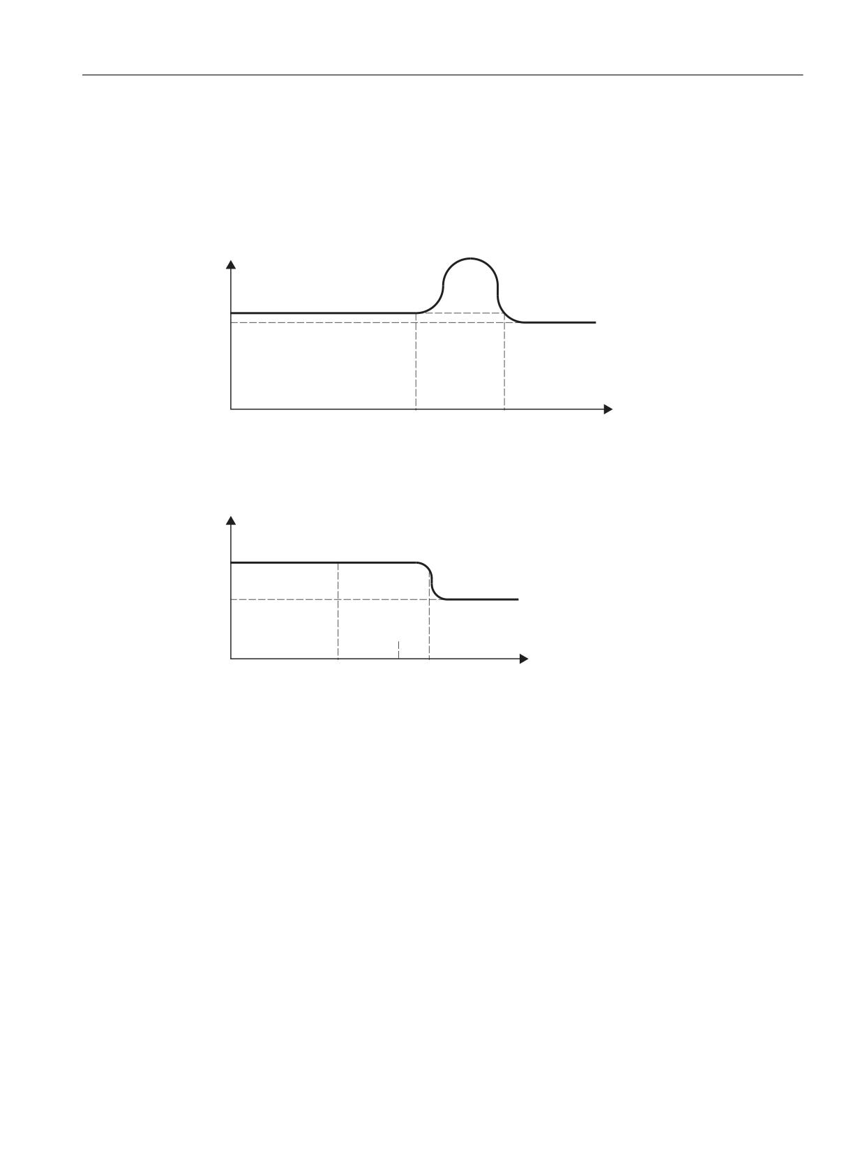
Continuous-path mode, exact stop, LookAhead
6.4 Dynamic adaptations
The minimum value of MD32440 for these three axes is thus 10 Hz. This means that any
acceleration, which is completed within a period of t2 - t1 = 2/10 Hz = 200 ms, is examined. The
time t2 is the time it takes to reach velocity v1 again following an acceleration process starting
from velocity v1. The extending of the execution time is also only considered within this range.
If the time t2 - t1 is greater than 200 ms or if the additional program execution time t3 - t2 is more
than 10% (= MD20460) of t2 - t1, the following time characteristic applies:
9
Y
Y
W
W
W
Figure 6-7
Characteristic of time-optimum path velocity (without smoothing)
If, however, the time t2 - t1 is less than 200 ms or if the additional program execution time t3 - t2
is no more than 10% of t2 - t1, the following time characteristic applies:
9
Y
Y
W
W
W
W
Figure 6-8
Characteristic of the smoothed path velocity
6.4.2
Adaptation of the dynamic path response
Function
Highly dynamic acceleration and deceleration processes during machining can cause excitation
of mechanical vibrations of machine elements and consequently a reduction of the surface
quality of the workpiece.
Basic functions
Function Manual, 10/2020, 6FC5397-2GP40-0BA1
475

Continuous-path mode, exact stop, LookAhead
6.4 Dynamic adaptations
The dynamic response of the acceleration and deceleration processes can be adapted to the
machine conditions using the "adaptation of the dynamic path response" function.
Note
The "adaptation of the dynamic path response" function only concerns the resulting path and
not the deceleration and acceleration processes of the individual axes involved in the path. For
this reason, critical deceleration and acceleration processes of the axes with respect to the
excitation of mechanical vibrations can occur due to discontinuous contour profiles or kinematic
transformations, even with a constant path velocity profile.
Effectiveness
The "adaptation of the dynamic path response" function is only effective during path motions:
• Continuous-path mode (G64, G64x)
In continuous-path mode, the optimal effect of the dynamic response adaptation is attained
with an active 100% override. Considerable deviations from this value or functions that cause
the path axes to decelerate (e.g. auxiliary function outputs to the PLC) greatly reduce the
desired action.
• Exact stop (G60)
In addition, the "adaptation of the dynamic path response" function is not active during path
motions:
• Programmed rapid traverse (G0)
• Changes in the override value
• Stop requests during motion (e.g. NC Stop, NC Reset)
• "Velocity-dependent path acceleration" function (DRIVE) is active
Activation/deactivation
The function is activated/deactivated with the machine data:
MD20465 $MC_ADAPT_PATH_DYNAMIC (adaptation of the dynamic path response)
Value
Meaning
= 1.0
Dynamic adaptation not active (default setting)
> 1.0
Dynamic adaptation active
When activation takes place, the "smoothing the path velocity" function is always activated
internally in continuous-path mode as well (see Section "Smoothing of the path velocity
(Page 472)").
If the smoothing factor (MD20460 $MC_LOOKAH_SMOOTH_FACTOR) is set to 0% (= function
deactivated; default!), a smoothing factor of 100% is used as a substitute. For a smoothing factor
other than 0%, the set value takes effect.
Basic functions
476
Function Manual, 10/2020, 6FC5397-2GP40-0BA1
Continuous-path mode, exact stop, LookAhead
6.4 Dynamic adaptations
Parameterization
Adaptation factor of the dynamic path response
Via the adaptation factor of the dynamic path response, temporary changes in the path velocity
are executed with smaller dynamic response limit values.
The adaptation factor is to be set on a channel-specific basis:
• For traversing motions with acceleration without jerk limitation (BRISK) via:
MD20465 $MC_ADAPT_PATH_DYNAMIC[ 0 ]
→ The adaptation factor acts on the acceleration.
• For traversing motions with acceleration with jerk limitation (SOFT) via:
MD20465 $MC_ADAPT_PATH_DYNAMIC[ 1 ]
→ The adaptation factor acts on the jerk.
Axis-specific limit frequencies
The dynamic response limiting should only be active during deceleration and acceleration
processes that trigger mechanical vibrations larger than a specific limiting frequency, thus
causing excitation of machine resonances.
This limit frequency from which the dynamic response limiting activates, is specified on an axis-
specific basis via the machine data:
MD32440 $MA_LOOKAH_FREQUENCY (smoothing frequency for LookAhead)
For further information, see Section "Smoothing of the path velocity (Page 472)".
Mode of operation
During processing and via all the axes involved in the path, the controller cyclically establishes
the minimum of all the limit frequencies to be the limit frequency (f) for the adaptation of the
dynamic response and calculates the relevant time window (tadapt) from this:
tadapt = 1 / f
The size of the relevant time window tadapt determines the further behavior:
1. The time needed to change the velocity is less than tadapt:
The acceleration rates are reduced by a factor > 1 and ≤ the value written in machine data:
MD20465 ADAPT_PATH_DYNAMIC (adaptation of the path dynamics)
The reduction in acceleration rate increases the time taken to change the velocity.
The following cases are different:
- The acceleration rate is reduced with a value less than MD20465 so that the process lasts
for tadapt [s]. The permitted reduction does not need to be fully utilized.
- The acceleration time is reduced with the value written in MD20465. The process lasts
less than tadapt despite the reduced acceleration. The permitted reduction was fully
utilized.
2. The time needed to change the velocity is greater than tadapt:
No dynamic response adaptation is required.
Basic functions
Function Manual, 10/2020, 6FC5397-2GP40-0BA1
477
Continuous-path mode, exact stop, LookAhead
6.4 Dynamic adaptations
Example
The following example is intended to show the effect of the "adaptation of the dynamic path
response" function on traversing motions with acceleration and without jerk limitation (BRISK).
The following parameters are assumed:
MD20465 $MC_ADAPT_PATH_DYNAMIC[0] = 1.5
MD20460 $MC_LOOKAH_SMOOTH_FACTOR = 1.0
MD32440 $MA_LOOKAH_FREQUENCY[AX1] = 20 Hz
TAX1 = 1/20 Hz = 50 ms
MD32440 $MA_LOOKAH_FREQUENCY[AX2] = 10 Hz
TAX2 = 1/10 Hz = 100 ms
MD32440 $MA_LOOKAH_FREQUENCY[AX3] = 20 Hz
TAX3 = 1/20 Hz = 50 ms
Note
To illustrate the effect of dynamic response adaptation, the value for the smoothing factor
(MD20460) is set to "1", whereby the "smoothing of the path velocity" function is practically
deactivated.
The path involves the three axes X = AX1, Y = AX2, Z = AX3.
For path motions in which axis AX2 is involved, all deceleration and acceleration processes that
would last less than TAX2 are adapted.
If only axes AX1 and/or AX3 are involved in path motions, all deceleration and acceleration
processes that would last less than TAX1 = TAX3 are adapted.
The relevant time window is marked tadapt... in the figures below.
Basic functions
478
Function Manual, 10/2020, 6FC5397-2GP40-0BA1
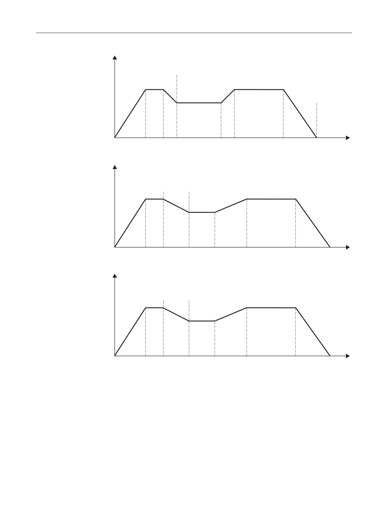
Continuous-path mode, exact stop, LookAhead
6.4 Dynamic adaptations
Y%
WDGDSW
Y
WDGDSW
WDGDSW
WDGDSW
W
W
W
W
W
W
W
W
W
Y%
WDGDSW
Y
WDGDSW
WDGDSW
W
W
W
W
W
W
W
W
W
Figure 6-9
Path velocity profile optimized for time without smoothing or dynamic adaptation response
Y%
WDGDSW
Y
WDGDSW
WDGDSW
W
W
W
W
W
W
W
W
W
Figure 6-10
Path velocity profile with adaptation of dynamic path response
Basic functions
Function Manual, 10/2020, 6FC5397-2GP40-0BA1
479

Continuous-path mode, exact stop, LookAhead
6.4 Dynamic adaptations
Intervals t
0
- t1 and t2 - t3:
The acceleration process between t0 - t1 and the deceleration
process between t2 - t3 are extended in terms of time to tadapt01
or tadapt23 as a result of the acceleration being adapted.
Interval t4 - t5:
The acceleration process between t4 - t5 is executed with an
acceleration reduced by the maximum adaptation factor of
1.5. However, the acceleration process is completed before
time tadapt45.
Interval t6 - t7:
The deceleration process between t6 - t7 remains unchanged as
it lasts longer than tadapt67.
6.4.3
Determination of the dynamic response limiting values
In addition to determining the natural frequency of the path axes for assigning parameters to the
axis-specific limit frequencies (MD32440 $MA_LOOKAH_FREQUENCY), the implementation of
the "adaptation of the dynamic path response" function also requires dynamic response limits to
be determined for velocity, acceleration and jerk.
Procedure
The determination of the dynamic response limits for the traversing of path axes by means of
acceleration with jerk limiting (SOFT) is described below. This procedure can be applied by
analogy to the case of acceleration without jerk limiting (BRISK).
1. Deactivate the "adaptation of the dynamic path response" function:
MD20465 $MC_ADAPT_PATH_DYNAMIC[1] = 1
2. Observe the positioning behavior of each path axis at different traversing velocities. When
doing so, set the jerk such that the desired positioning tolerance is maintained.
Note
The higher the traversing velocity from which the positioning process is started, the higher
in general the jerk can be set.
3. Use the maximum permissible jerk determined for the least critical traversing velocity:
MD32431 $MA_MAX_AX_JERK (maximum jerk)
4. Determine the FAPD factor for all of the path axes using:
FAPD = (largest determined jerk) / (smallest determined jerk)
Note
The smallest determined jerk is the value for the jerk during the most critical traversing
velocity.
5. Enter the largest FAPD factor that was determined via all the path axes as the value for the
adaptation factor for the path dynamic response:
MD20465 $MC_ADAPT_PATH_DYNAMIC[ 1 ] = FAPD
Basic functions
480
Function Manual, 10/2020, 6FC5397-2GP40-0BA1