SINUMERIK 840D sl/828D. Job Planning. Programming Manual (2010-2018) - page 4
File and Program Management
3.1 Program memory
Example:
The workpiece directory _N_SHAFT_WPD, created for SHAFT workpiece contains the
following files:
File
Description
_N_SHAFT_MPF
Main program
_N_PART2_MPF
Main program
_N_PART1_SPF
Subprogram
_N_PART2_SPF
Subprogram
_N_SHAFT_INI
General initialization program for the data of the workpiece
_N_SHAFT_SEA
Setting data initialization program
_N_PART2_INI
General initialization program for the data for the Part 2 program
_N_PART2_UFR
Initialization program for the frame data for the Part 2 program
_N_SHAFT_COM
Comment file
Data can also be stored in the workpiece directory which is not directly required by the NC for
the machining. In addition to ASCII files, this can be binary files, such as images in JPG format
or descriptions in PDF format. In order that these can be interpreted as binary files by the NC,
the file extensions must be known in the NC (setting during commissioning via MD17000 $MN_
EXTENSIONS_OF_BIN_FILES; the following file extensions are preset in the basic setting:
JPG, GIF, PNG, BMP, PDF, ICO, HTM).
Select workpiece for machining
A workpiece directory can be selected for execution in a channel. If a main program with the
same name or only a single main program (_MPF) is stored in this directory, this is automatically
selected for execution.
References:
Operating Manual
3.1.2
External program memory
In addition to the passive file system in the NC, external program memories can also be
available at the machine (e.g. on the local drive or on a network drive).
Using the functions "Execute from external" or "EES (Execution from External Storage)" part
programs can be directly executed from external program memories.
Reference:
Function Manual Basic Functions; K1: Mode Group, Channel, Program Operation, Reset
Response
Global part program memory (GDIR)
When declaring the drives, one of the drives can be designated the global part program
memory (GDIR).
References:
Operating Manual: section: "Manage programs" > "Setting up drives"
Job Planning
Programming Manual, 12/2018, A5E40869460B AB
213
File and Program Management
3.1 Program memory
The system automatically creates the MPF.DIR, SPF.DIR and WKS.DIR directories on the
drive. These three directories form the GDIR.
The GDIR only plays a role for the EES function. Depending on the drive configuration, the
GDIR replaces or extends the NC part program memory. The creation of a GDIR is, however,
not essential for EES operation.
The directories and files of the GDIR can be addressed in the part program in the same way
as in the passive file system. This permits a compatible transfer of an NC program with path
details from the passive file system to the GDIR. The directory SPF.DIR of the GDIR is
contained in the search path for subprograms.
Program organization
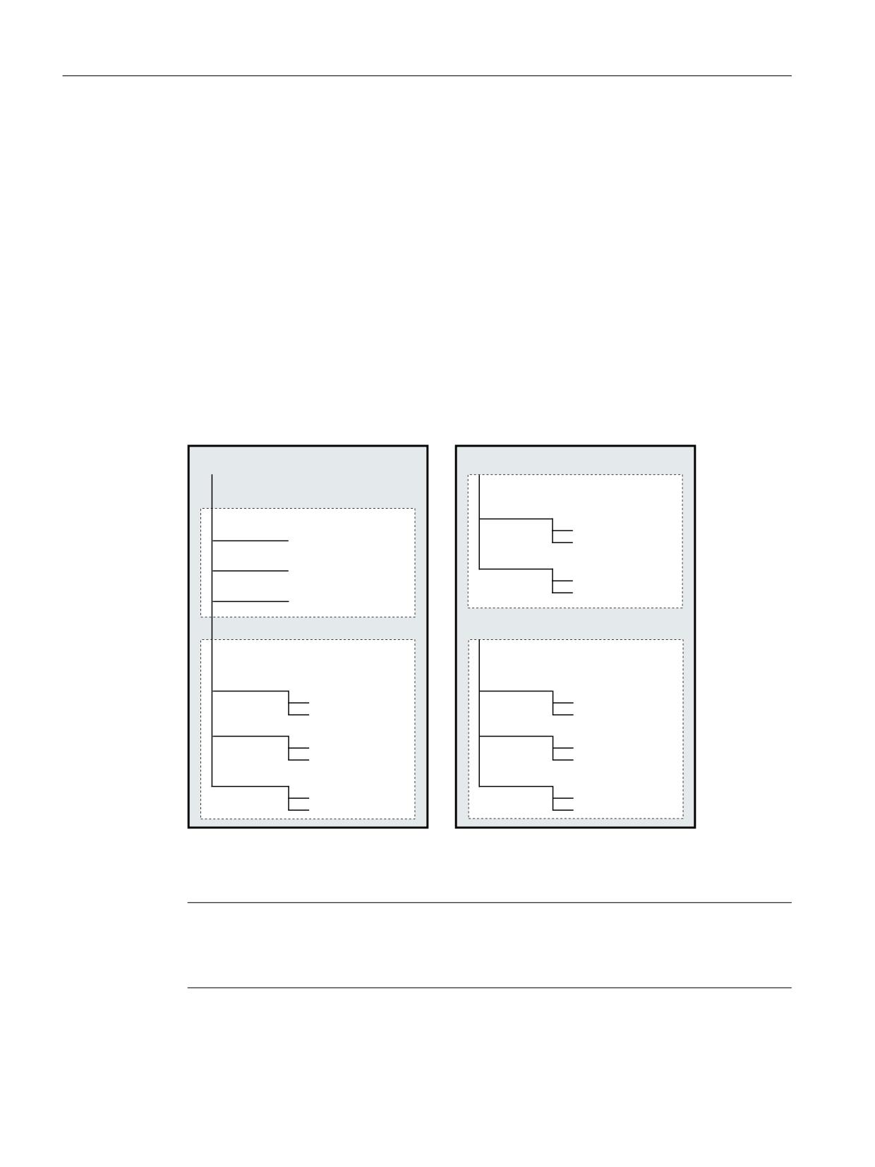
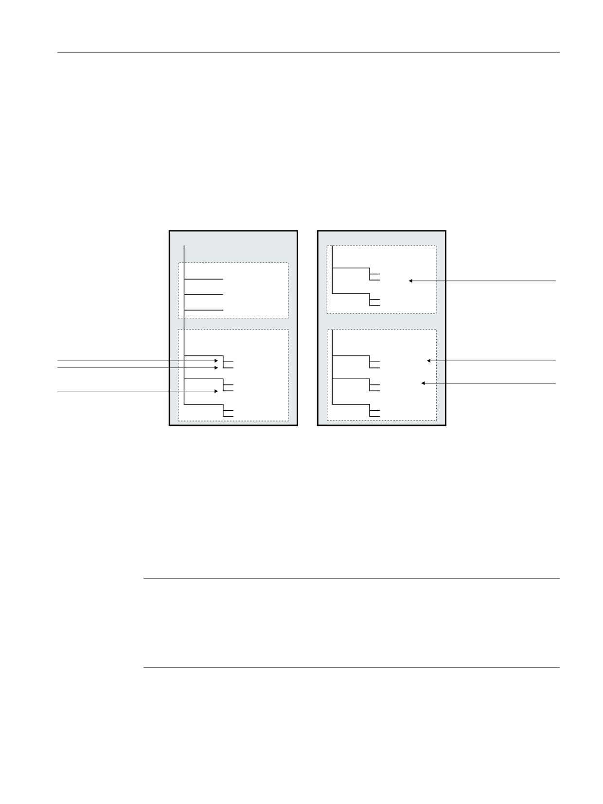
The program organization on external program memories is shown in the following diagram:
3DVVLYH ILOH V\VWHP LQ WKH 1&.
([WHUQDO SURJUDP PHPRU\
'(9
$Q\ GULYH
3URJV
&\FOHV
0\3URJ 0SI
B1B&67B',5
SS
[[[
B1B&0$B',5
PRUH3URJV
6+$)7
B1B&86B',5
0\6XE3 63)
'(9
3DUW SURJUDP PHPRU\
*OREDO SDUW SURJUDP
PHPRU\ *',5
03) ',5
03) ',5
B1B352* B03)
352*
03)
B1B352* B03)
352*
03)
63) ',5
63) ',5
B1B68% B63)
68%
63)
B1B68% B63)
68%
63)
:.6 ',5
:.6 ',5
Case-insensitive file systems
Note
To avoid problems with case-sensitivity for the file addressing (see "Addressing program
memory files (Page 215)"), case-insensitive file systems should be used as external program
memory.
Job Planning
214
Programming Manual, 12/2018, A5E40869460B AB
File and Program Management
3.1 Program memory
3.1.3
Addressing program memory files
A file in the program memory, which is addressed with a file handling command (e.g. WRITE,
DELETE, READ, ISFILE, FILEDATE, FILETIME, FILESIZE, FILESTAT, FILEINFO), is
referenced with an absolute path plus file names or only with the file names. In the second
case, the path of the selected program is used as file path.
Addressing in the NC/EES notation
3DVVLYH ILOH V\VWHP LQ WKH 1&.
([WHUQDO SURJUDP PHPRU\
'(9
DQ\ GULYH
3URJV
&\FOHV
B1B&67B',5
0\3URJ 0SI
SS
[[[
$GGUHVVLQJ LQ WKH ((6 QRWDWLRQ
B1B&0$B',5
PRUH3URJV
'(9
3URJV SS
[[[
6+$)7
B1B&86B',5
0\6XE3 63)
'(9
3DUW SURJUDP PHPRU\
*OREDO SDUW SURJUDP
PHPRU\ *',5
$GGUHVVLQJ LQ WKH 1&. QRWDWLRQ
$GGUHVVLQJ LQ WKH 1&. QRWDWLRQ
B1B03)B',5
03) ',5
B1B03)B',5 B1B352* B03)
B1B03)B',5 B1B352* B03)
B1B352* B03)
352*
03)
B1B352* B03)
352*
03)
$GGUHVVLQJ LQ WKH ((6 QRWDWLRQ
B1B63)B',5
63) ',5
03) ',5 352* 03)
B1B68% B63)
68%
63)
$GGUHVVLQJ LQ WKH ((6 QRWDWLRQ
B1B68% B63)
68%
63)
([SOLFLW DGGUHVVLQJ
'(9
63) ',5 68%
63)
B1B:.6B',5
:.6 ',5
1& B1B63)B',5 B1B68% B63)
RU
1& 63) ',5 68%
63)
Addressing files of the passive file system
Files of the passive file system are generally addressed in the NC notation (directory and file
names begin with the domain identifier "_N_", "_" is the separator for the file identifier) without
specifying the drive name. An addressing in EES notation (without domain identification "_N_",
separator for the directory/file extension is ".") is, however, also permitted.
Example:
● NC notation: "/_N_SPF_DIR/_N_SUB1_SPF"
● EES notation: "/SPF.DIR/SUB1.SPF"
Note
The addressing schemes for files of the passive file system in EES notation are converted
internally into NC notation in accordance with the following rules:
● Directory and file names are extended with the domain identification "_N_".
● If the fourth-last character in the directory or file name is a period ("."), it will be converted
into an underscore ("_").
The passive file system can also be explicitly addressed using the predefined drive names "//
NC:".
Job Planning
Programming Manual, 12/2018, A5E40869460B AB
215
File and Program Management
3.1 Program memory
Example:
● NC notation: "//NC:/_N_SPF_DIR/_N_SUB1_SPF"
● EES notation: "//NC:/SPF.DIR/SUB1.SPF"
Addressing files of an external program memory
Files of an external program memory not recorded as GDIR must be addressed in EES
notation. The drive name (e.g. "//DEV1:") must be specified at the start of the addressing path.
All symbolic device names configured in /user/sinumerik/hmi/cfg/logdrive.ini are permissible.
Example:
● EES notation: "//DEV1:/MyProgDir/pp1.xxx"
● NC notation: Not permissible
Addressing files of the global part program memory (GDIR)
When addressing files of the GDIR, in addition to specifying the path in the EES notation, it is
also permissible to specify the path in the NC notation.
Example:
● EES notation: "//DEV2:/MPF.DIR/PROG11.MPF"
● NC notation: "/_N_MPF_DIR/_N_PROG11_MPF"
Note
The addressing schemes for files of the GDIR in NC notation are converted internally into EES
notation in accordance with the following rules:
● The domain identification "_N_" in directory and file names is removed.
● If the fourth-last character in the directory or file name is an underscore ("_"), it will be
converted into a period (".").
Rules for the path specification
A complete path specification consists of drive name, directory path and file name.
Drive name
The following rules govern the specification of the drive name:
● All symbolic device names configured in /user/sinumerik/hmi/cfg/logdrive.ini are
permissible.
● The character "//" is at the beginning, followed by at least one letter or one digit.
● The following characters can be any combination of letters, digits, "_" and spaces.
● The name is ended with a letter or a digit, followed by a ":".
● Other special characters are not permitted.
Job Planning
216
Programming Manual, 12/2018, A5E40869460B AB
File and Program Management
3.1 Program memory
Note
The drive name "//NC:" is predefined for the passive file system.
Examples:
● External program memory:
-
//Drive1:
–
//Drive_1:
–
//Drive 1:
–
//A B:
–
//1 B C 2:
Directory path
The following rules govern the specification of the directory path:
● A "/" is located at the start and end of the directory path and as separator for the individual
path sections.
Note
A double slash ("//") within the directory path is not permitted!
● Directory names:
- Directory names must begin with a letter or a digit. Only for addressing in the NC notation
do directory names begin with the domain identification "_N_".
- The following characters can be any combination of letters, digits and "_".
Note
Spaces in directory names are also permitted for external program memories. This is
not true, however, when the external program memory is created as global part program
memory (GDIR).
- Other special characters are not permitted.
● Directory extensions:
- Directory extensions must consist of three letters/digits.
- They are separated with "_" (NC notation) or "." (EES notation) from the directory name.
Note
The passive file system has only the directory extensions _DIR and _WPD.
Job Planning
Programming Manual, 12/2018, A5E40869460B AB
217
File and Program Management
3.1 Program memory
Examples:
● Passive file system or GDIR:
- NC notation: _N_WKS_DIR/_N_MYNCPROGS_WPD/...
- EES notation: WKS.DIR/MYPROGS.WPD/...
● External program memory:
- /abc
- /ab_c.def
- /ab c1.def
- /a b c .d11
- /abc.def/ghi.klm
File name
The following rules apply to the file names:
● Only for addressing in NC notation do file names begin with the domain identification "_N_".
● The next two characters should be either two letters or an underscore followed by a letter.
Note
If this condition is satisfied, then an NC program can be called as subprogram from another
program just by specifying the program name. However, if the program name starts with
digits, the subprogram call is then only possible via the CALL statement.
● The following characters can be any combination of letters, digits and "_".
● File extension:
- The file extension must consist of three letters/digits.
Note
Permitted file extensions in the passive file system, see "NC program memory
(Page 211)".
- They are separated with "_" (NC notation) or "." (EES notation) from the file names.
Examples:
● Passive file system or GDIR:
- NC notation: _N_SUB1_SPF
- EES notation: SUB1.SPF
● External program memory:
- Part 1
- _Part1
- Part_1.spf
- Part1.mpf
Job Planning
218
Programming Manual, 12/2018, A5E40869460B AB
File and Program Management
3.1 Program memory
DIN subprogram name
The following rules apply to DIN subprogram names:
● The first character must be the letter "L".
● The following characters are digits (at least one).
● File extension:
- The file extension must consist of three letters.
- They are separated with "_" (NC notation) or "." (EES notation) from the file names.
Examples:
● L123
● L1_SPF (NC notation) or L1.SPF (EES notation)
Maximum path length
Maximum 128 bytes are available for specifying the drive name and the directory path; the
maximum length of the file name is 31 bytes. The maximum length of the complete path is
159 bytes.
3.1.4
Search path for subprogram call
For subprogram calls without path data, the absolute path is determined by processing a fixed
search path.
A search is then made in the program memory in the following sequence:
Directory
Description
1
current directory / name
The current directory is the directory in which the
program is selected.
2
current directory / name_SPF
This can be:
3
current directory / name_MPF
● A workpiece directory or the standard
directory _N_MPF_DIR in the NC part
program memory or global part program
memory
or
● Any directory of an external program memory
4
a
//NC:/_N_SPF_DIR / name_SPF
Subprogram directory in the NC part program
memory
b
//DEV2:/_N_SPF_DIR / name_SPF 1)
Subprogram directory in the global part program
memory
Note:
This search step is not executed if a global part
program memory has not been created, or the
program is selected in the NC part program
memory.
Job Planning
Programming Manual, 12/2018, A5E40869460B AB
219

File and Program Management
3.1 Program memory
Directory
Description
5
Search path extension programmed with CALLPATH (see "Extend search path for subprogram
calls (CALLPATH) (Page 199)").
Note:
This search step is not executed if CALLPATH has not been programmed.
6
/_N_CUS_DIR / name_SPF
User cycle directory
7
/_N_CMA_DIR / name_SPF
Manufacturer cycle directory
8
/_N_CST_DIR / name_SPF
Standard cycle directory
1)
//DEV2:" For example represents the drive on which the global part program memory has been
created.
The following rules apply for the search:
● The search path is run through for each individual subprogram call, this means that it is
irrelevant where the higher-level program is located.
● Depending on the directory, different file types are taken into account.
● A search is made in a directory, and not in lower-level, i.e. nested directories.
3.1.5
Interrogating the path and file name
The following system variables, which can be read in the part program, are available to
interrogate the path and file name of an NC program:
System variable
Type
Meaning
$P_STACK
INT
Supplies the program level in which the current NC program
is executed.
$P_PATH[ <n>]
STRING
Supplies the path of the NC program, which is processed at
the program level selected using field index <n>.
Examples:
$P_PATH[0] supplies the path for the main program, e.g. "/
_N_WKS_DIR/_N_WELLE_WPD/".
$P_PATH[$P_STACK - 1] supplies the path of the calling pro-
gram.
If the path refers to an NC program, which is saved in the pas-
sive file system of the NC or in the global part program memory
(GDIR), then the path is supplied in the NC notation.
If the path refers to an NC program, which is executed by an
external program memory other than the global part program
memory then $P_PATH supplies the path in the EES notation.
$P_PROG[ <n>]
STRING
Supplies the name of the NC program, which is processed at
the program level selected using field index <n>.
If the NC program is saved in the passive file system of the NC
or in the global part program memory, then the program name
is supplied in the NC notation.
If the NC program is executed by an external drive other than
the global part program memory, then $P_PROG supplies the
name in the EES notation.
Job Planning
220
Programming Manual, 12/2018, A5E40869460B AB

File and Program Management
3.1 Program memory
System variable
Type
Meaning
$P_PROGPATH
STRING
Supplies the path of the NC program that is presently being
processed.
Calling $P_PROGPATH is identical to $P_PATH[$P_STACK].
$P_IS_EES_PATH[ <n>]
BOOL
Interrogates whether the path supplied by $P_PATH[<n>] or
the program name supplied by $P_PROG[<n>] corresponds
to the NC notation or the EES notation.
= FALSE
$P_PATH[<n>] and $P_PROG[<n>] supply a NC
notation. This means that each identifier has the
prefix "_N_". The separator for the file identifier is
"_".
Examples:
● Path in the NC notation: "/_N_WKS_DIR/
_N_MYWPD_WPD/"
● Program name in the NC
notation:"_N_MYPROG_MPF"
A path in the NC notation can refer to the passive
file system in the NC as well as also the global part
program memory.
= TRUE
$P_PATH[<n>] and $P_PROG[<n>] supply an
EES notation. This means that the identifiers do
not have the "_N_" prefix. The separator for the file
identifier is ".".
Examples:
● Path in the EES notation: "//DEV1:/WKS.DIR/
MYWPD.WPD/"
● Program name in the EES notation:
"MYPROG.MPF"
<n>: Index <n> defines the program level, from which the path information should be read (value range:
0 ... 17)
Note
In the EES mode, outside the global part program memory (GDIR), system variables
$P_PROG, $P_PATH and $P_PROGPATH path names in the EES notation. For the EES
mode, user programs that evaluate and process these path names must be extended so that
they can also process pathnames in the EES notation.
Job Planning
Programming Manual, 12/2018, A5E40869460B AB
221

File and Program Management
3.2 Working memory (CHANDATA, COMPLETE, INITIAL)
3.2
Working memory (CHANDATA, COMPLETE, INITIAL)
Function
The working memory contains the current system and user data with which the control is
operated (active file system), e.g.:
● Active machine data
● Tool offset data
● Zero offsets
● ...
Initialization programs
These are programs with which the working memory data is initialized. The following file types
can be used for this:
File type
Description
name_TEA
Machine data
name_SEA
Setting data
name_TOA
Tool offsets
name_UFR
Zero offsets/frames
name_INI
Initialization files
name_GUD
Global user data
name_RPA
R-parameters
Data areas
The data can be organized in different areas in which they are to apply. For example, a control
can have several channels or, as is commonly the case, several axes at its disposal.
There are:
Identifier
Data areas
NC
NC-specific data
CH<n>
Channel-specific data (<n> specifies the channel name)
AX<n>
Axis-specific data (<n> specifies the number of the machine axis)
TO
Tool data
COMPLETE
All data
Job Planning
222
Programming Manual, 12/2018, A5E40869460B AB
File and Program Management
3.2 Working memory (CHANDATA, COMPLETE, INITIAL)
Create initialization program at an external PC
The data area identifier and the data type identifier can be used to determine the areas which
are to be treated as a unit when the data is saved:
_N_AX5_TEA_INI
Machine data for axis 5
_N_CH2_UFR_INI
Frames of channel 2
_N_COMPLETE_TEA_INI
All machine data
When the control is started up initially, a set of data is automatically loaded to ensure proper
operation of the control.
Procedure for multi-channel controls (CHANDATA)
CHANDATA(<channel number>) for several channels is only permissible in the file
_N_INITIAL_INI. This is the commissioning file with which all data of the control is initialized.
Program code
Comment
%_N_INITIAL_INI
CHANDATA(1)
; Machine axis assignment, channel 1:
$MC_AXCONF_MACHAX_USED[0]=1
$MC_AXCONF_MACHAX_USED[1]=2
$MC_AXCONF_MACHAX_USED[2]=3
CHANDATA(2)
; Machine axis assignment, channel 2:
$MC_AXCONF_MACHAX_USED[0]=4
$MC_AXCONF_MACHAX_USED[1]=5
CHANDATA(1)
; Axial machine data:
; Exact stop window coarse:
$MA_STOP_LIMIT_COARSE[AX1]=0.2
; Axis 1
$MA_STOP_LIMIT_COARSE[AX2]=0.2
; Axis 2
; Exact stop window fine:
$MA_STOP_LIMIT_FINE[AX1]=0.01
; Axis 1
$MA_STOP_LIMIT_FINE[AX1]=0.01
; Axis 2
NOTICE
CHANDATA statement
In the part program, the CHANDATA statement may only be set for that channel in which the
NC program is executed. This means the statement can be used to protect NC programs so
that they are not executed in the wrong channel.
Program processing is aborted if an error occurs.
Job Planning
Programming Manual, 12/2018, A5E40869460B AB
223
File and Program Management
3.2 Working memory (CHANDATA, COMPLETE, INITIAL)
Note
INI files in job lists do not contain any CHANDATA statements.
Save initialization program (COMPLETE, INITIAL)
The files of the working memory can be saved on an external PC and then read in again from
there.
● The files are saved with COMPLETE.
● INITIAL is used to create an INI file (_N_INITIAL_INI) over all areas.
Read-in initialization program
NOTICE
Data loss
If the file is read-in with the name "INITIAL_INI", then all data that is not supplied in the file is
initialized using standard data. Only machine data is an exception. This means that setting
data, tool data, ZO, GUD values, ... are supplied with standard data (normally "ZERO").
For example, the file COMPLETE_TEA_INI is suitable for reading-in individual machine data.
The control only expects machine data in this file. This is the reason that the other data areas
remain unaffected in this case.
Loading initialization programs
The INI programs can also be selected and called as part programs if they only use data of
one channel. This means that it is also possible to initialize program-controlled data.
Job Planning
224
Programming Manual, 12/2018, A5E40869460B AB

Protection zones
4
4.1
Defining protection zones (CPROTDEF, NPROTDEF)
Protection zones, which protect machine elements against collisions, are defined in the part
program in blocks. These contain the following elements:
1. Definition of the machining plane
Before the actual protection zone definition, the machining plane must be selected, to which
the contour description of the protection zone refers.
2. Start of the definition
Depending on the particular NC command, either a channel-specific or machine-specific
protection zone is created.
3. Contour description of the protection zone
The contour of a protection zone is defined with traversing motion. These are not executed
and have no connection to previous or subsequent geometry descriptions. They only define
the protection zone.
4. End of definition
Syntax
DEF INT <Var>
G17/G18/G19
CPROTDEF/NPROTDEF(<n>,<t>,<AppLim>,<AppPlus>,<AppMinus>)
G0/G1/... X/Y/Z
EXECUTE(<Var>)
Meaning
DEF INT <Var>:
Definition of a local help variable, of the INTEGER data type
<Var>:
Name of the Help variable
G17/G18/G19:
Machining plane
Note:
It is not permissible to change the machining plane before the
end of the definition. Programming the applicate is not permitted
between start and end of the definition.
CPROTDEF():
Predefined procedure to define a channel-specific protection
zone
NPROTDEF():
Predefined procedure to define a machine-specific protection
zone
<n>:
Number of defined protection zone
Data type:
INT
Job Planning
Programming Manual, 12/2018, A5E40869460B AB
225
Protection zones
4.1 Defining protection zones (CPROTDEF, NPROTDEF)
<t>:
Type of protection zone
Data type:
BOOL
Value:
TRUE
Tool-related protection zone
FALSE
Workpiece-related protection zone
<AppLim>:
Type of limitation in the third dimension
Data type:
INT
Value:
0
No limitation
1
Limit in plus direction
2
Limit in minus direction
3
Limit in positive and negative direction
<AppPlus>:
Value of the limit in the positive direction in the 3rd dimension
Data type:
REAL
<AppMinus>:
Value of the limit in the negative direction in the 3rd dimension
Data type:
REAL
G0/G1/... X/Y/Z
:
The contour of a protection zone is specified with up to 11 tra-
versing movements in the selected machining plane. The first
traversing movement is the movement to the contour. The last
point in the contour description must always coincide with the
first point of the contour description.
The valid protection zone is the zone left of the contour:
● Internal protection zone
The contour of an internal protection zone must described
in the counterclockwise direction.
● External protection zones (permitted only for workpiece-
related protection zones)
The contour for an external protection zone must be
described in the clockwise direction.
The following contour elements are permissible:
● G0, G1 for straight contour elements
● G2 for circle segments in the clockwise direction
Permissible only for workpiece-related protection zones.
Not permissible for tool-related protection zones because
they must be convex.
● G3 for circular segments in the counter-clockwise direction
Note:
A protection zone cannot be described by a complete circle. A
complete circle must be divided into two semicircles.
Note:
The sequence G2 → G3 or G3 → G2 is not permissible! A short
G1 block must be inserted between the two circular blocks.
EXECUTE(<Var>):
Predefined procedure that marks the end of the definition
A switch is made back to normal program processing with
EXECUTE.
Example
See example under "Activating/deactivating protection zones (CPROT, NPROT) (Page 229)".
Job Planning
226
Programming Manual, 12/2018, A5E40869460B AB
Protection zones
4.1 Defining protection zones (CPROTDEF, NPROTDEF)
Additional information
Machine-specific protection zones
A machine-specific protection zone or its contour is defined using the geometry axis, i.e.
referenced to the basic coordinate system (BCS) of a channel. In order that correct protection-
zone monitoring can take place in all channels in which the machine-specific protection zone
is active, the basic coordinate system (BCS) of all of the channels involved must be identical:
● position of the coordinate origin referred to the machine zero
● Orientation of the coordinate axes
Reference point for contour description
● Tool-related protection zones
Coordinates for tool-related protection zones must be specified as absolute values referred
to the tool holder reference point F.
● Workpiece-related protection zones
Coordinates for workpiece-related protection zones must be specified as absolute values
referred to the zero point of the basic coordinate system (BCS).
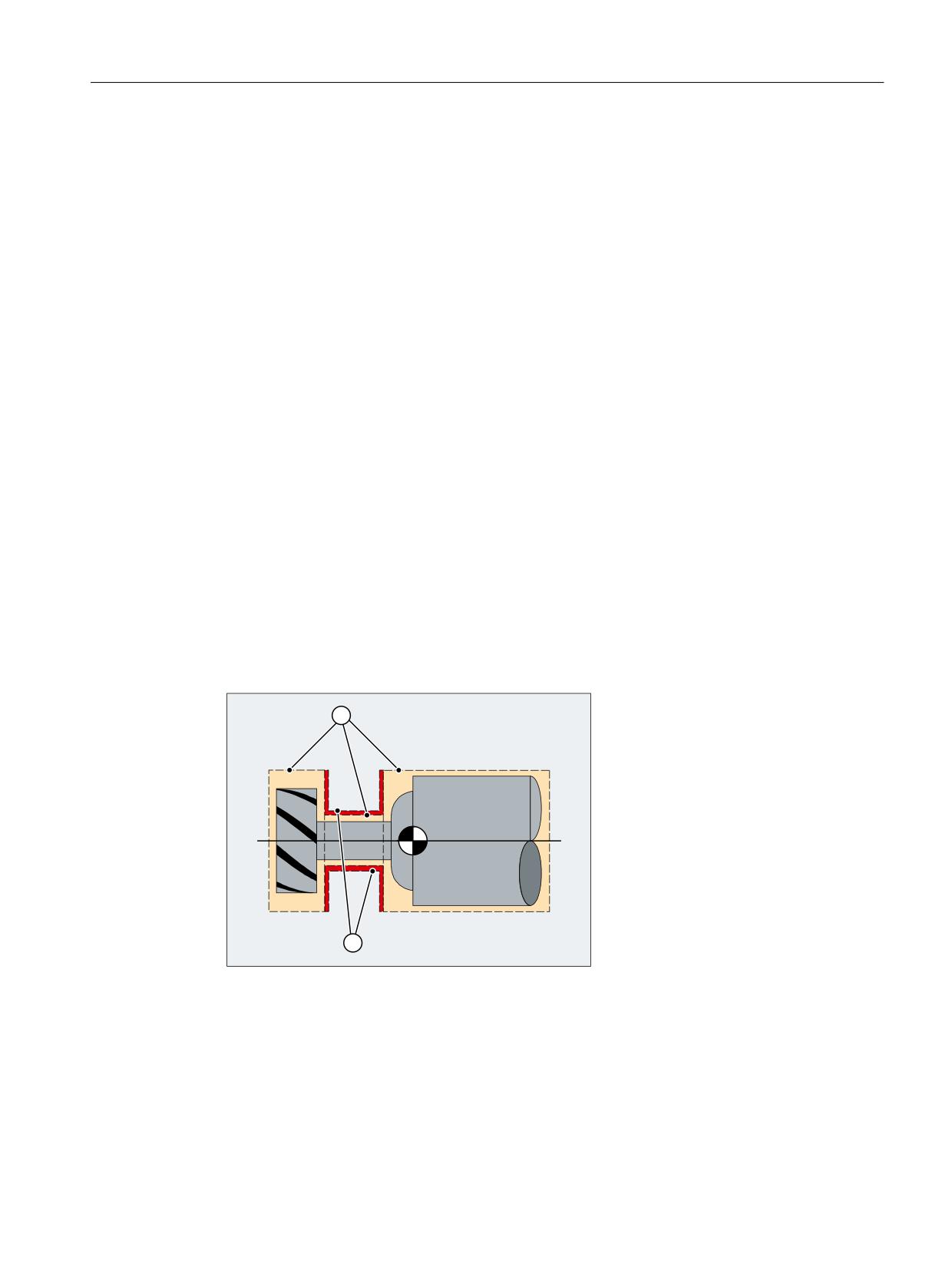
Protection zones symmetrical around the center of rotation
For protection zones symmetrical around the axis or rotation (e.g. spindle chuck), you must
describe the complete contour and not only the contour up to the center of rotation.
Tool-related protection zones
Tool-related protection zones must always be convex. If a concave protected zone is desired,
this should be subdivided into several convex protection zones.
)
① Convex protection zones
② Concave protection zones (not permissible!)
F Toolholder reference point
Job Planning
Programming Manual, 12/2018, A5E40869460B AB
227
Protection zones
4.1 Defining protection zones (CPROTDEF, NPROTDEF)
General conditions
During the definition of a protection zone, the following functions must not be active or used:
● Tool radius compensation (cutter radius compensation, tool nose radius compensation)
● Transformation
● Reference point approach (G74)
● Fixed point approach (G75)
● Dwell time (G4)
● Block search stop (STOPRE)
● End of program (M17, M30)
● M functions: M0, M1, M2
Job Planning
228
Programming Manual, 12/2018, A5E40869460B AB
Protection zones
4.2 Activating/deactivating protection zones (CPROT, NPROT)
4.2
Activating/deactivating protection zones (CPROT, NPROT)
Protection zones previously defined in the part program can be activated at any time - or can
be preactivated for subsequent activation by the PLC user program. Active protection zones
can be deactivated at any time.
When activating or preactivating, it is also possible to relatively shift the reference point of the
protection zone.
Note
A protection zone is only taken into account after the referencing of all geometry axes of the
channel in which it has been activated.
Note
Monitoring protection zones
If a tool-related protection area is not active, the tool path is checked against the workpiece-
related protection zones.
If no workpiece-oriented protection zone is active, then there is no protection zone monitoring.
Syntax
CPROT(<n>,<Status>,<XMov>,<YMov>,<ZMov>)
NPROT(<n>,<Status>,<XMov>,<YMov>,<ZMov>)
Meaning
CPROT:
Predefined procedure to activate a channel-specific protection
zone
NPROT:
Predefined procedure to activate a machine-specific protection
zone
<n>:
Number of the protection zone
Data type:
INT
<Status>:
The channel-specific activation status is set using this parameter
Data type:
INT
Value:
0
Deactivate protection zone
1
Preactivate protection zone
2
Activate protection zone
3
Preactivate protection zone with conditional
stop
<XMov>,<YMov>,<ZMov>:
Additive offset values in the X/Y/Z direction
The offset can take place in 1, 2, or 3 dimensions. The offset values
refer to:
● The machine zero for a workpiece-related protection zone
● The tool carrier reference point F for a tool-specific protection
zone
Data type:
REAL
Job Planning
Programming Manual, 12/2018, A5E40869460B AB
229
Protection zones
4.2 Activating/deactivating protection zones (CPROT, NPROT)
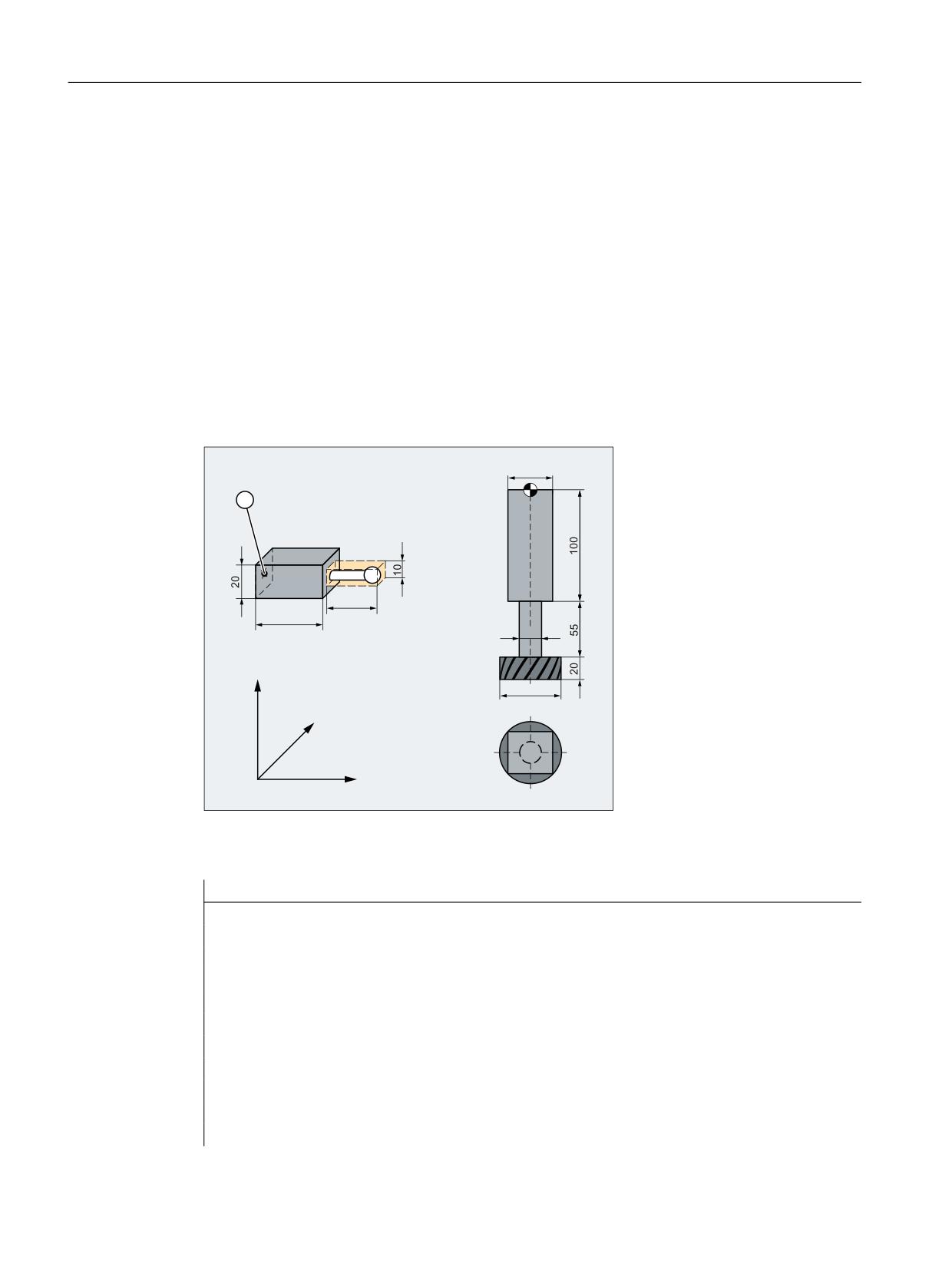
Example
Possible collision of a milling cutter with the measuring probe is to be monitored on a milling
machine. The position of the measuring probe is to be defined by an offset when the function
is activated.
The following protection zones are defined for this:
● A machine-specific and a workpiece-related protection zone for both the measuring probe
holder (n-PZ1) and the measuring probe itself (n-PZ2).
● A channel-specific and a tool-related protection zone for the milling cutter holder (c-PZ1),
the cutter shank (c-PZ2) and the milling cutter itself (c-PZ3).
The orientation of all protection zones is in the Z direction.
The position of the reference point of the measuring probe on activation of the function must
be X = -120, Y = 60 and Z = 80.
)
Q 3=
Q 3=
F 3=
F 3=
F 3=
=
<
;
① Name for the protection zone of the probe
F
Toolholder reference point
Program code
Comment
DEF INT PROTZONE
; Definition of a Help variable
G17
; machining plane XY
; defining protection zones:
NPROTDEF(1,FALSE,3,10,-10)
; protection zone n-PZ1
G01 X0 Y-10
X40
Y10
X0
Y-10
EXECUTE(PROTZONE)
Job Planning
230
Programming Manual, 12/2018, A5E40869460B AB
Protection zones
4.2 Activating/deactivating protection zones (CPROT, NPROT)
Program code
Comment
NPROTDEF(2,FALSE,3,5,-5)
;
protection zone n-PZ2
G01 X40 Y-5
X70
Y5
X40
Y-5
EXECUTE(PROTZONE)
CPROTDEF(1,TRUE,3,0,-100)
;
protection zone c-PZ1
G01 X-20 Y-20
X20
Y20
X-20
Y-20
EXECUTE(PROTZONE)
CPROTDEF(2,TRUE,3,-100,-150)
;
protection zone c-PZ2
G01 X0 Y-10
G03 X0 Y10 J10
X0 Y-10 J-10
EXECUTE(PROTZONE)
CPROTDEF(3,TRUE,3,-150,-170)
;
protection zone c-PZ3
G01 X0 Y-27.5
G03 X0 Y27.5 J27.5
X0 Y27.5 J-27.5
EXECUTE(PROTZONE)
; activating protection zones:
NPROT(1,2,-120,60,80)
;
activate protection zone n-PZ1 with offset
NPROT(2.2,-120,60,80)
;
activate protection zone n-PZ2 with offset
CPROT(1,2,0,0,0)
;
activate protection zone c-PZ1
CPROT(2,2,0,0,0)
;
activate protection zone c-PZ2
CPROT(3,2,0,0,0)
;
activate protection zone c-PZ3
Further information
Activation status after the control powers up
A protection zone can already be active after the control system powers up and the axes have
been referenced. This is the case if, for the protection zone, the following system variable is
set to TRUE:
● $SN_PA_ACTIV_IMMED[<n>] (for machine-specific protection zone) or
● $SC_PA_ACTIV_IMMED[<n>] (for channel-specific protection zone)
Index "<n>" corresponds to the number of the protection zone: 0 = 1. Protection zone
The protection zone is activated with status = 2 - and without offset.
Job Planning
Programming Manual, 12/2018, A5E40869460B AB
231
Protection zones
4.2 Activating/deactivating protection zones (CPROT, NPROT)
Multiple activation of a protection zone
A machine-specific protection zone can be active simultaneously in several channels (e.g.
protection zone of a tailstock where there are two opposite sides). The protection zones are
only monitored if all geometry axes have been referenced.
A protection zone cannot be activated simultaneously with different offsets in a single channel.
Protection zone monitoring for active tool radius compensation
For active tool radius compensation, a functioning protection zone monitoring is only possible
if the plane of the tool radius compensation is identical to the plane of the protection zone
definitions.
Job Planning
232
Programming Manual, 12/2018, A5E40869460B AB
Protection zones
4.3 Checking for protection zone violation, working area limitation and software limit switches (CALCPOSI)
4.3
Checking for protection zone violation, working area limitation and
software limit switches (CALCPOSI)
Function
In the workpiece coordinate system (WCS), the CALCPOSI function checks whether, starting
from the starting position, the geometry axes can be traversed a specified distance without
violating active limits. For the case that the distance cannot be fully traversed because of limits,
a positive, decimal-coded status value and the maximum possible traversing distance are
returned.
Definition
INT CALCPOSI(VAR REAL[3] <Start>, VAR REAL[3] <Dist>, VAR REAL[5]
<Limit>, VAR REAL[3] <MaxDist>, BOOL <MeasSys>, INT <TestLim>)
Syntax
<Status> = CALCPOSI(VAR <Start>, VAR <Dist>, VAR <Limit>, VAR
<MaxDist>, <MeasSys>, <TestLim>)
Meaning
CALCPOSI(...):
Predefined function for testing limit violations regarding the geometry axes
Preprocessing
No
stop:
Alone in the block:
Yes
Job Planning
Programming Manual, 12/2018, A5E40869460B AB
233
Protection zones
4.3 Checking for protection zone violation, working area limitation and software limit switches (CALCPOSI)
<status>:
Function return value. Negative values indicate error states.
(Part 1)
Data type:
INT
Value range:
-8 ≤ x ≤ 100000
Value:
0
The distance can be traversed completely.
-1
At least one component is negative in <Limit>.
-2
Error in a transformation calculation.
Example: The traversing distance passes through a singu-
larity so that the axis positions cannot be defined.
-3
The specified traversing distance <Dist> and the maximum
possible traversing distance <MaxDist> are linearly depend-
ent.
Note
Can only occur in conjunction with <TestLim>, bit 4 == 1.
-4
The projection of the traversing direction contained in <Dist>
on to the limitation surface is the zero vector, or the traversing
direction is perpendicular to the violated limitation surface.
Note
Can only occur in conjunction with <TestLim>, bit 5 == 1.
-5
In <TestLim>, bit 4 == 1 AND bit 5 == 1
-6
At least one machine axis that has to be considered for
checking the traversing limits has not been referenced.
-7
Collision avoidance function: Invalid definition of the kine-
matic chain or the protection zones.
-8
Collision avoidance function: This command cannot be exe-
cuted because of insufficient memory.
<status>:
Units digit
(Part 2)
Note
If several limits are violated simultaneously, the limit with the greatest restriction
on the specified traversing distance is signaled.
Value:
1
Software limit switches are limiting the traversing distance
2
Working area limits are limiting the traversing distance
3
Protection zones are limiting the traversing distance
4
Collision avoidance function: Protection zones are limiting
the traversing path
Tens digit
Value:
1x
The initial value violates the limit
2x
The specified straight line violates the limit.
This value is returned even if the end point does not violate
any limit itself, but the path from the starting point to the end
point would cause a limit value to be violated (e.g. by passing
through a protection zone, curved software limit switches in
the WCS for non-linear transformations, e.g. transmit).
Job Planning
234
Programming Manual, 12/2018, A5E40869460B AB
Protection zones
4.3 Checking for protection zone violation, working area limitation and software limit switches (CALCPOSI)
<status>:
Hundreds digit
(Part 3)
Value:
1xx
AND units digit == 1 or 2:
The positive limit value has been violated.
AND units digit == 3 1):
An NC-specific protection zone has been violated.
2xx
AND units digit == 1 or 2:
The negative limit value has been violated.
AND units digit == 3 1):
A channel-specific protection zone is violated.
<status>:
Thousands digit
(Part 4)
Value:
1xxx
AND units digit == 1 or 2:
Factor with which the axis number is multiplied that violates
the limit. Numbering of the axes begins with 1.
Reference:
● Software limit switches: Machine axes
● Working area limitation: Geometry axes
AND units digit == 3 1):
Factor with which the number of the violated protection zone
is multiplied.
<status>:
Hundred thousands digit
(Part 5)
Value:
0xxxxx
Hundred thousands digit == 0: <Dist> remains unchanged
1xxxxx
A direction vector is returned in <Dist>, which defines the
further motion direction on the limitation surface.
Can only occur with the following supplementary conditions:
● Software limit switch or working area limit violated (not in
the starting point)
● A transformation is not active
● <TestID>, bit 4 or bit 5 == 1
<Start>:
Reference to a vector with the start positions:
● <Start> [0]: 1st geometry axis
● <Start> [1]: 2nd geometry axis
● <Start> [2]: 3rd geometry axis
Parameter type:
Input
Data type:
VAR REAL [3]
Value range:
-max. REAL value ≤ x[<n>] ≤ +max. REAL value
Job Planning
Programming Manual, 12/2018, A5E40869460B AB
235
Protection zones
4.3 Checking for protection zone violation, working area limitation and software limit switches (CALCPOSI)
<Dist>:
Reference to a vector.
Input: Incremental traversing distance
● <Dist> [0]: 1st geometry axis
● <Dist> [1]: 2nd geometry axis
● <Dist> [2]: 3rd geometry axis
Output (only for set hundred thousands digit in <Status>):
<Dist> contains a unit vector v as output value which defines the further tra-
versing direction in the WCS.
Case 1: Formation of vector v for <TestID>, bit 4 == 1
The input vectors <Dist> and <MaxDist> span the motion plane. This plane
is cut by the violated limitation surface. The intersecting line of the two planes
defines the direction of vector v.The orientation (sign) is selected so that the
angle between the input vector <MaxDist> and v is not greater than 90 de-
grees.
Case 2: Formation of vector v for <TestID>, bit 5 == 1
Vector v is the unit vector in the projection direction of the traversing vector
contained in <Dist> on the limitation surface. If the projection of the traversing
vector on the limitation surface is the zero vector, an error is returned.
Parameter type:
Input/output
Data type:
VAR REAL [3]
Value range:
-max. REAL value ≤ x[<n>] ≤ +max. REAL value
<Limit>:
Reference to an array of length 5.
● <Limit> [0 - 2]: Minimum clearance of the geometry axes to the limits:
- <Limit> [0]: 1st geometry axis
- <Limit> [1]: 2nd geometry axis
- <Limit> [2]: 3rd geometry axis
The minimum clearances are observed with:
- Working area limitation: No restrictions
- Software limit switches: If no transformation is active, or a transformation
is active in which a clear assignment of the geometry axes to the linear
machine axes is possible, e.g. 5-axis transformations.
● <Limit> [3]: Contains the minimum clearance for linear machine axes which,
for example, cannot be assigned a geometry axis because of a non-linear
transformation. This value is also used as limit value for the monitoring of the
conventional protection zones and the collision avoidance protection zones.
● <Limit> [4]: Contains the minimum clearance for rotary machine axes which,
for example, cannot be assigned a geometry axis because of a non-linear
transformation.
Note
This value is only active for the monitoring of the software limit switches for
special transformations.
Parameter type:
Input
Data type:
VAR REAL [5]
Value range:
-max. REAL value ≤ x[n] ≤ +max. REAL value
Job Planning
236
Programming Manual, 12/2018, A5E40869460B AB
Protection zones
4.3 Checking for protection zone violation, working area limitation and software limit switches (CALCPOSI)
<MaxDist>:
Reference to a vector with the incremental traversing distance in which the speci-
fied minimum clearance of an axis limit is not violated by any of the relevant ma-
chine axes:
● <Dist> [0]: 1st geometry axis
● <Dist> [1]: 2nd geometry axis
● <Dist> [2]: 3rd geometry axis
If the traversing distance is not restricted, the contents of this return parameter
are the same as the contents of <Dist>.
For <TestID>, bit 4 == 1: <Dist> and <MaxDist>
<MaxDist> and <Dist> must contain vectors as input values that span a motion
plane. The two vectors must be mutually linearly independent. The absolute value
of <MaxDist> is arbitrary. For the calculation of the motion direction, see the de-
scription for <Dist>.
Parameter type:
Output
Data type:
VAR REAL [3]
Value range:
-max. REAL value ≤ x[<n>] ≤ +max. REAL value
<MeasSys>:
Measuring system (inch/metric) for position and distance specifications (optional)
Data type:
BOOL
Value:
FALSE
System of units corresponding to the currently active G com-
mand from the G group 13 (G70, G71, G700, G710).
(De-
fault)
Note
If G70 is active and the basic system is metric (or G71 is
active and the basic system is inch), the system variables
$AA_IW and $AA_MW are provided in the basic system and,
if used, must be converted for CALCPOSI.
TRUE
System of units according to the set basic system:
MD52806 $MN_ISO_SCALING_SYSTEM
<TestLim>:
Bit-coded selection of the limits to be monitored (optional)
Data type:
INT
Default value:
Bits 0, 1, 2, 3, 6, 7 == 1 (207)
Bit
Decimal
Meaning
0
1
Software limit switch
1
2
Working area limitation
2
4
Activated conventional protection zones
3
8
Preactivated conventional protection zones
4
16
With violated software limit switches or working area limits in
<Dist>, return the traversing direction as in Case 1 (see
above).
5
32
With violated software limit switches or working area limits in
<Dist>, return the traversing direction as in Case 2 (see
above).
6
64
Activated collision avoidance protection zones
7
128
Preactivated collision avoidance protection zones
8
256
Pairs of activated and preactivated collision avoidance pro-
tection zones
1) If several protection zones are violated, the protection zone with the greatest restriction on the speci-
fied traversing distance is returned.
Job Planning
Programming Manual, 12/2018, A5E40869460B AB
237
Protection zones
4.3 Checking for protection zone violation, working area limitation and software limit switches (CALCPOSI)
Example
Limitations
<
6RIWZDUH OLPLW VZLWFK
&
1
1
:RUNLQJ DUHD OLPLWDWLRQ
1
1
1
&
;
1
1
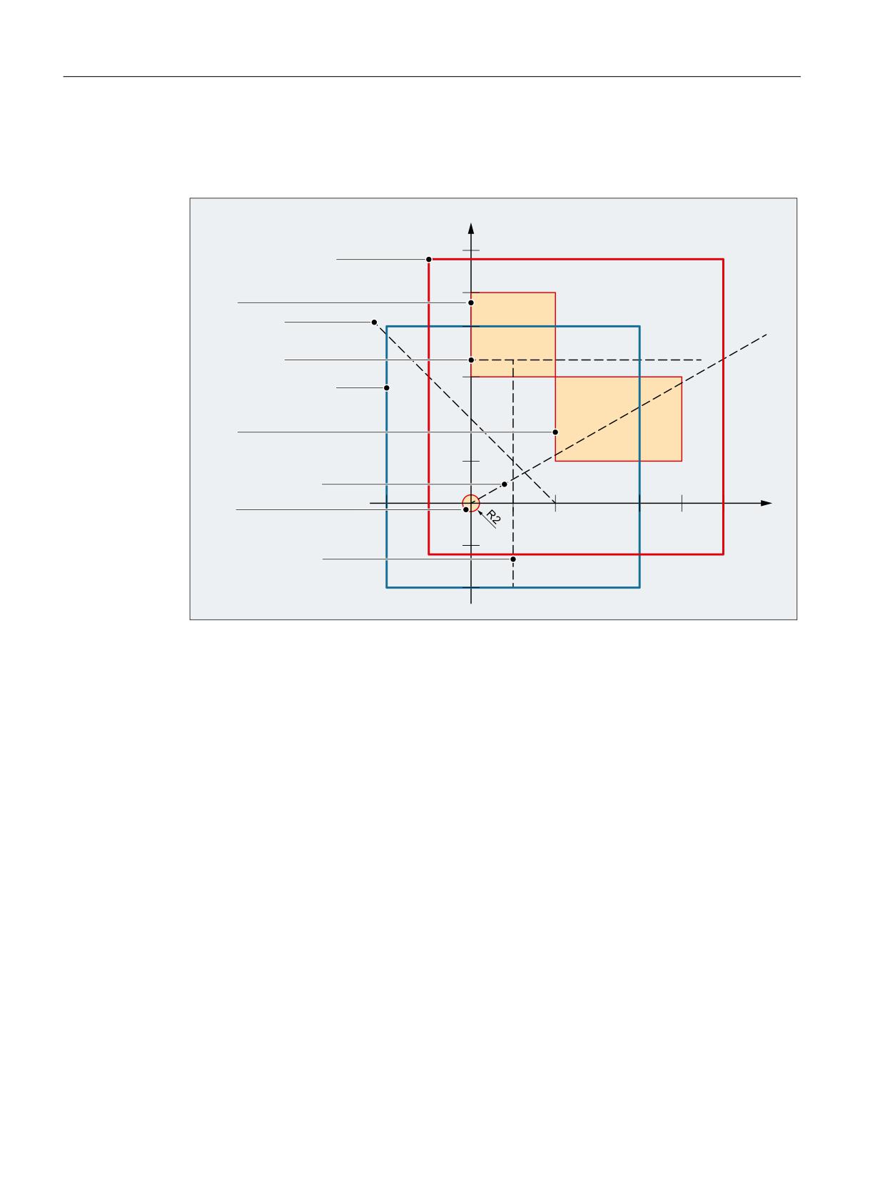
In the example, the active software limit switches and working area limits in the X-Y plane and
the following three protection zones are displayed:
● C2: Tool-related, channel-specific protection zone, active, circular, radius = 2 mm
● C4: Workpiece-related, channel-specific protection zone, preactivated, square, side length
= 10 mm
● N3: Machine-specific protection zone, active, rectangular, side length = 10 mm x 15 mm
NC program
The protection zones and working area limits are defined first in the NC program. The
CALCPOSI() function is then called with different parameter assignments.
Program code
N10 DEF REAL _START[3]
N20 DEF REAL _DIST[3]
N30 DEF REAL _LIMIT[5]
N40 DEF REAL _MAXDIST[3]
N50 DEF INT _PA
N60 DEF INT _STATUS
Job Planning
238
Programming Manual, 12/2018, A5E40869460B AB
Protection zones
4.3 Checking for protection zone violation, working area limitation and software limit switches (CALCPOSI)
Program code
: toolrelated protection zone C2
N70 CPROTDEF(2, TRUE, 0)
N80 G17 G1 X-2 Y0
N90 G3 I2 X2
N100 I-2 X-2
N110 EXECUTE(_PA)
; workpiece-related protection zone C4
N120 CPROTDEF(4, FALSE, 0)
N130 G17 G1 X0 Y15
N140 X10
N150 Y25
N160 X0
N170 Y15
N180 EXECUTE(_PA)
; machine-specific protection zone N3
N190 NPROTDEF(3, FALSE, 0)
N200 G17 G1 X10 Y5
N210 X25
N220 Y15
N230 X10
N240 Y5
N250 EXECUTE(_PA)
; activate or preactivate protection zones
N260 CPROT(2, 2, 0, 0, 0)
N270 CPROT(4, 1, 0, 0, 0)
N280 NPROT(3, 2, 0, 0, 0)
; define working area limits
N290 G25 XX=-10 YY=-10
N300 G26 XX=20 YY=21
N310 _START[0] = 0.
N320 _START[1] = 0.
N330 _START[2] = 0.
N340 _DIST[0] = 35.
N350 _DIST[1] = 20.
N360 _DIST[2] =
0.
N370 _LIMIT[0] = 0.
N380 _LIMIT[1] = 0.
N390 _LIMIT[2] = 0.
N400 _LIMIT[3] = 0.
N410 _LIMIT[4] = 0.
N420 _STATUS = CALCPOSI(_START, _DIST, _LIMIT, _MAXDIST)
N430 _STATUS = CALCPOSI(_START, _DIST, _LIMIT, _MAXDIST,,3)
N440 _STATUS = CALCPOSI(_START, _DIST, _LIMIT, _MAXDIST,,1)
N450 _START[0] =
5.
N460 _START[1] = 17.
N470 _START[2] =
0.
N480 _DIST[0] =
0.
N490 _DIST[1] =-27.
N500 _DIST[2] =
0.
N510 _STATUS = CALCPOSI(_START, _DIST, _LIMIT, _MAXDIST,,14)
N520 _STATUS = CALCPOSI(_START, _DIST, _LIMIT, _MAXDIST,, 6)
N530 _LIMIT[1] = 2.
Job Planning
Programming Manual, 12/2018, A5E40869460B AB
239

Protection zones
4.3 Checking for protection zone violation, working area limitation and software limit switches (CALCPOSI)
Program code
N540 _STATUS = CALCPOSI(_START, _DIST, _LIMIT, _MAXDIST,, 6)
N550 _START[0] = 27.
N560 _START[1] = 17.1
N570 _START[2] =
0.
N580 _DIST[0] =-27.
N590 _DIST[1] =
0.
N600 _DIST[2] =
0.
N610 _LIMIT[3] = 2.
N620 _STATUS = CALCPOSI(_START, _DIST, _LIMIT, _MAXDIST,,12)
N630 _START[0] = 0.
N640 _START[1] = 0.
N650 _START[2] = 0.
N660 _DIST[0] =
0.
N670 _DIST[1] = 30.
N680 _DIST[2] =
0.
N690 TRANS X10
N700 AROT Z45
N710 _STATUS = CALCPOSI(_START,_DIST, _LIMIT, _MAXDIST)
; delete frames from N690 and N700 again
N720 TRANS
N730 _START[0] =
0.
N740 _START[1] = 10.
N750 _START[2] =
0.
; vectors_DIST and _MAXDIST define the motion plane
N760 _DIST[0] = 30.
N770 _DIST[1] = 30.
N780 _DIST[2] =
0.
N790 _MAXDIST[0] = 1.
N800 _MAXDIST[1] = 0.
N810 _MAXDIST[2] = 1.
N820 _STATUS = CALCPOSI(_START, _DIST, _LIMIT, _MAXDIST,,17)
N830 M30
Results of CALCPOSI()
N...
<status>
<MaxDist>[0] ≙ X
<MaxDist>[1] ≙ Y
Remarks
420
3123
8.040
4.594
N3 is violated.
430
1122
20.000
11.429
No protection zone monitoring,
working area limitation is violated.
440
1121
30.000
17.143
Only software limit monitoring is still active.
510
4213
0.000
0.000
Starting point violates C4
520
0000
0.000
-27.000
Preactivated C4 is not monitored. The
specified distance can be traversed com-
pletely.
540
2222
0.000
-25.000
Because _LIMIT[1] = 2, the traversing dis-
tance is restricted by the working area limi-
tation.
Job Planning
240
Programming Manual, 12/2018, A5E40869460B AB

Protection zones
4.3 Checking for protection zone violation, working area limitation and software limit switches (CALCPOSI)
N...
<status>
<MaxDist>[0] ≙ X
<MaxDist>[1] ≙ Y
Remarks
620
4223
-13.000
0.000
Clearance to C4 is a total of 4 mm due to
C2 and _LIMIT[3]. Clearance C2 → N3 of
0.1 mm does not result in limitation of the
traversing distance.
710
1221
0.000
21.213
Frame with translation and rotation active.
The permissible traversing distance in
_DIST applies in the shifted and rotated
WCS.
820
102121
18.000
18.000
The software limit switch of the Y axis is
violated. The calculation of a further tra-
versing direction is requested with <_TES-
TLIM> = 17. This direction is in _DIST
(0.707, 0.0, 0.707). It is valid because the
hundred thousands digit is set in <_STA-
TUS>.
Additional information
"Referenced" axis status
All machine axes considered by CALCPOSI() must be homed.
Circle-related distance specifications
All circle-related distance specifications are always interpreted as radius specifications. This
must be taken into account particularly for transverse axes with activated diameter
programming (DIAMON/DIAM90).
Traversing distance reduction
If the specified traversing distance of an axis is limited, the traversing distance of the other
axes is also reduced proportionally in the <MaxDist> return value. The resulting end point is
therefore still on the specified path.
Rotary axes
Rotary axes are only monitored when they are not modulo rotary axes.
It is permissible that no software limit switches, working area limits or protection zones are
defined for one or more of the relevant axes.
Software limit switch and working area limitation status
Software limit switches and working area limits are only taken into account if they are active
during the execution of CALCPOSI(). The status can be influenced, for example, via:
● Machine data: MD21020 $MC_WORKAREA_WITH_TOOL_RADIUS
● Setting data: $AC_WORKAREA_CS_...
● NC/PLC interface signals DB31, ... DBX12.2 / 3
● Commands: WALIMON / WALIMOF
Job Planning
Programming Manual, 12/2018, A5E40869460B AB
241
Protection zones
4.3 Checking for protection zone violation, working area limitation and software limit switches (CALCPOSI)
Software limit switches and transformations
With CALCPOSI(), the positions of the machine axes (MCS) cannot always be uniquely
determined from the positions of the geometry axes (WCS) during various kinematic
transformations (e.g. TRANSMIT) because of ambiguities at certain positions of the traversing
distance. In normal traversing operation, the uniqueness generally results from the history and
the condition that a continuous motion in the WCS must correspond to a continuous motion in
the MCS. Therefore, when monitoring the software limit switches, the machine position at the
time when CALCPOSI() is executed is used to resolve the ambiguity in such cases.
Note
Preprocessing stop
When using CALCPOSI() in conjunction with transformations, it is the sole responsibility of
the user to program a preprocessing stop (STOPRE) with the preprocessing before
CALCPOSI() for the synchronization of the machine axis positions.
Protection zone clearance and conventional protection zones
With conventional protection zones, there is no guarantee that the safety clearance set in
parameter <Limit>[3] is maintained for all protection zones during a traversing movement
on the specified path. It is only guaranteed that no protection zone will be violated when the
end point returned in <Dist> is extended by the safety clearance in the traversing direction.
However, the straight line can pass very close to a protection zone.
Protection zone clearance and collision avoidance protection zones
With collision avoidance protection zones, there is a guarantee that the safety clearance set
in parameter <Limit>[3] is maintained for all protection zones during a traversing movement
on the specified traversing path.
The safety clearance specified in parameter <Limit>[3] only takes effect when the following
applies:
<Limit>[3] > (MD10619 $MN_COLLISION_TOLERANCE)
If bit 4 is set in parameter <TestLim> (calculation of the ongoing traversing direction), then
the direction vector received in <DIST> is only valid when the hundred thousands digit is set
in the function return value (<status>). If a direction such as this cannot be determined, either
because protection zones were violated, or because a transformation is active, then the input
value in <DIST> remains unchanged. An additional error message is not output.
Job Planning
242
Programming Manual, 12/2018, A5E40869460B AB

Special motion commands
5
5.1
Approaching coded positions (CAC, CIC, CDC, CACP, CACN)
You can traverse linear and rotary axes via position numbers to fixed axis positions saved in
machine data tables using the following commands. This type of programming is called
"approach coded positions".
Syntax
CAC(<n>)
CIC(<n>)
CACP(<n>)
CACN(<n>)
Meaning
CAC(<n>):
Approach coded position from position number n
CIC(<n>):
Starting from the actual position number, approach the coded position n position
locations before (+n) or back (-n)
CDC(<n>):
Approach the position from position number n along the shortest path
(only for rotary axes)
CACP(<n>):
Approach coded position from position number n in the positive direction
(only for rotary axes)
CACN(<n>):
Approach coded position from position number n in the negative direction
(only for rotary axes)
<n>:
Position number within the machine data table
Range of values: 0, 1, … (max. number of table locations - 1)
Example: Approach coded positions of a positioning axis
Programming code
Comment
N10 FA[B]=300
; Feedrate for positioning axis B
N20 POS[B]=CAC(10)
; Approach coded position from position number 10
N30 POS[B]=CIC(-4)
; Approach coded position from "current position num-
ber" - 4
References
● Function Manual Expanded Functions; Indexing Axes (T1)
● Function Manual, Synchronized Actions
Job Planning
Programming Manual, 12/2018, A5E40869460B AB
243
Special motion commands
5.2 Spline interpolation (ASPLINE, BSPLINE, CSPLINE, BAUTO, BNAT, BTAN, EAUTO, ENAT, ETAN, PW, SD,
PL)
5.2
Spline interpolation (ASPLINE, BSPLINE, CSPLINE, BAUTO, BNAT,
BTAN, EAUTO, ENAT, ETAN, PW, SD, PL)
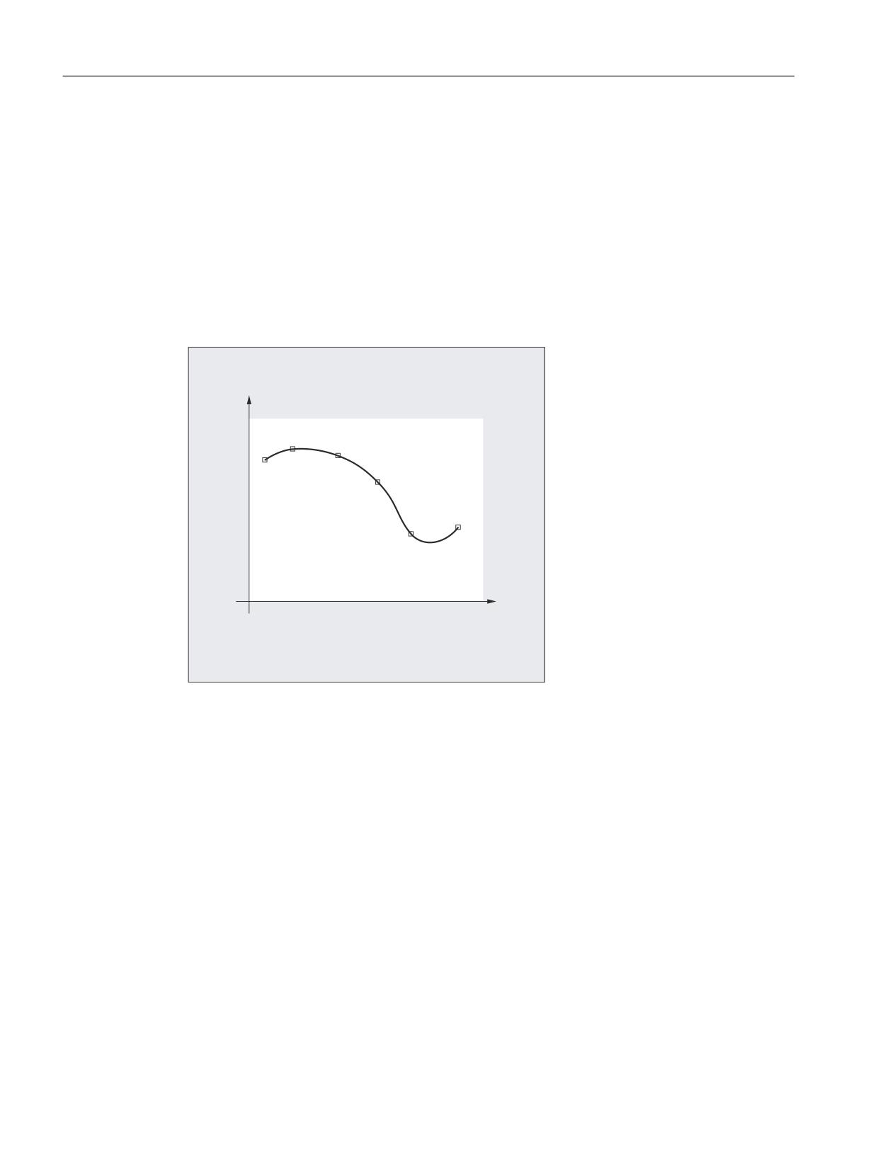
Randomly curved workpiece contours cannot be precisely defined in an analytic form. This is
the reason why these type of contours are approximated using a limited number of points along
curves, e.g. when digitizing surfaces. The points along the curve must be connected to define
a contour in order to generate the digitized surface of a workpiece. Spline interpolation permits
this.
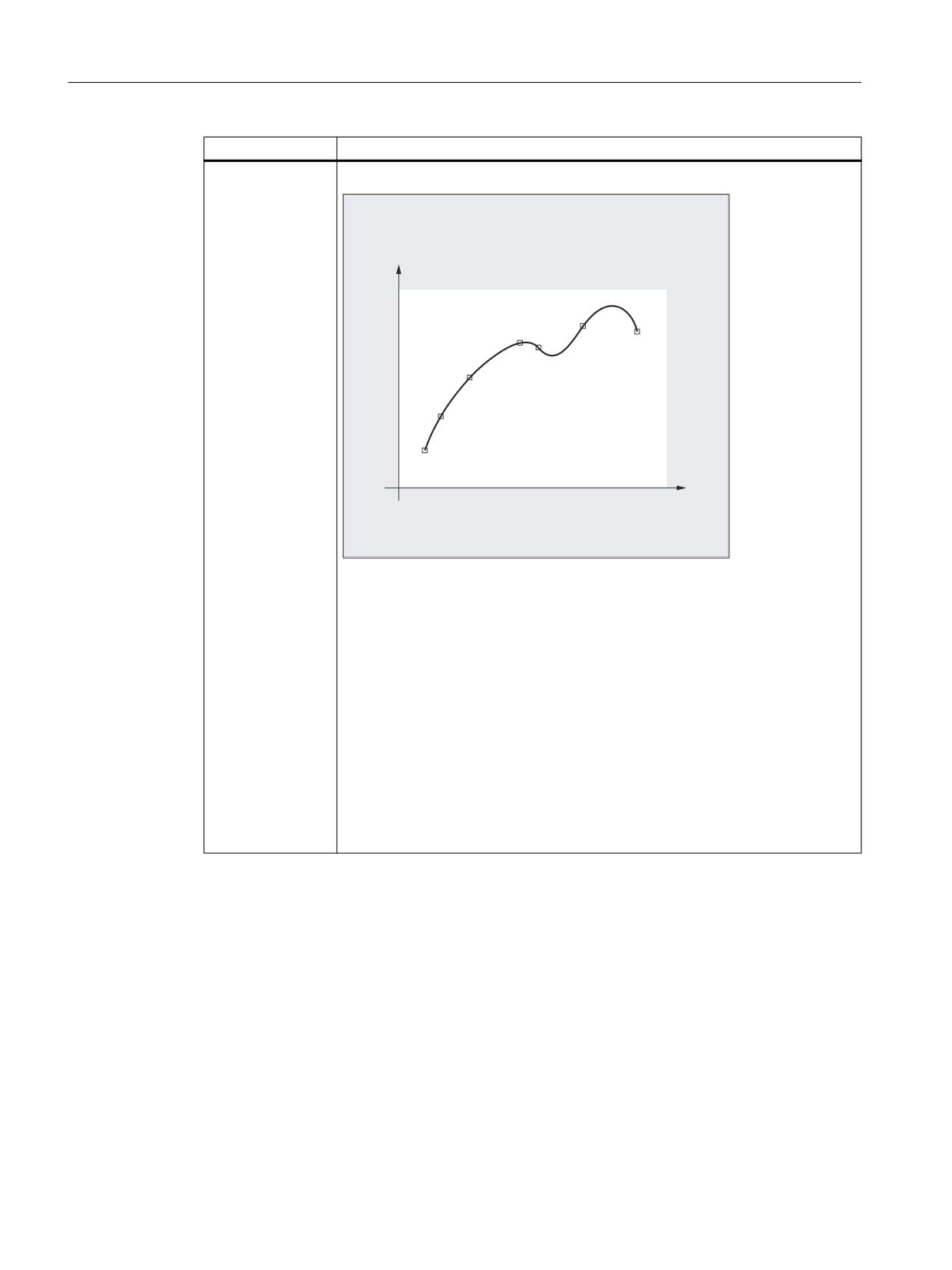
A spline defines a curve which is formed from polynomials of 2nd or 3rd degree. The
characteristics of the points along the curve of a spline can be defined depending on the spline
type being used.
3
3
3
3
3
3
3
WR 3
VSHFLILHG FRRUGLQDWHV
For SINUMERIK solution line, the following spline types are available:
● A spline
● B spline
● C spline
Syntax
General:
ASPLINE X... Y... Z... A... B... C...
BSPLINE X... Y... Z... A... B... C...
CSPLINE X... Y... Z... A... B... C...
For a B spline, the following can be additionally programmed:
PW=<n>
SD=2
PL=<value>
For A and C splines, the following can be additionally programmed:
BAUTO / BNAT / BTAN
Job Planning
244
Programming Manual, 12/2018, A5E40869460B AB
Special motion commands
5.2 Spline interpolation (ASPLINE, BSPLINE, CSPLINE, BAUTO, BNAT, BTAN, EAUTO, ENAT, ETAN, PW, SD,
PL)
EAUTO / ENAT / ETAN
Meaning
Spline interpolation type:
ASPLINE:
Command to activate A spline interpolation
BSPLINE:
Command to activate B spline interpolation
CSPLINE:
Command to activate C spline interpolation
The ASPLINE, BSPLINE and CSPLINE commands are modally effective
and belong to the group of motion commands.
Points along a curve and check points:
X... Y... Z...
Positions in Cartesian coordinates
A... B... C...
Point weight (only B spline):
PW:
Using the PW command, a so-called "point weight" can be programmed for
every point along the curve.
<n>:
"Point weight"
Range of values:
0 ≤ n ≤ 3
Increment:
0.0001
Effect:
n > 1
The checkpoint attracts the curve more
significantly.
n < 1
The checkpoint attracts the curve less sig-
nificantly.
Spline degree (only B spline):
SD:
A third degree polygon is used as standard, However, a second degree
polygon can also be used by programming SD=2.
Distance between nodes (only B spline):
PL :
The distances between nodes are suitably calculated internally. The control
can also machine pre-defined node clearances that are specified in the so-
called parameter-interval-length using the PL command.
<value>:
Parameter interval length
Range of values:
As for path dimension
Transitional behavior at the start of the spline curve (only A or C spline):
BAUTO:
No specifications for the transitional behavior. The start is determined by
the position of the first point.
BNAT:
Zero curvature
BTAN:
Tangential transition to the previous block (delete position)
Transitional behavior at the end of the spline curve (only A or C spline):
EAUTO:
No specifications for the transitional behavior. The end is determined by
the position of the last point.
ENAT:
Zero curvature
Job Planning
Programming Manual, 12/2018, A5E40869460B AB
245
Special motion commands
5.2 Spline interpolation (ASPLINE, BSPLINE, CSPLINE, BAUTO, BNAT, BTAN, EAUTO, ENAT, ETAN, PW, SD,
PL)
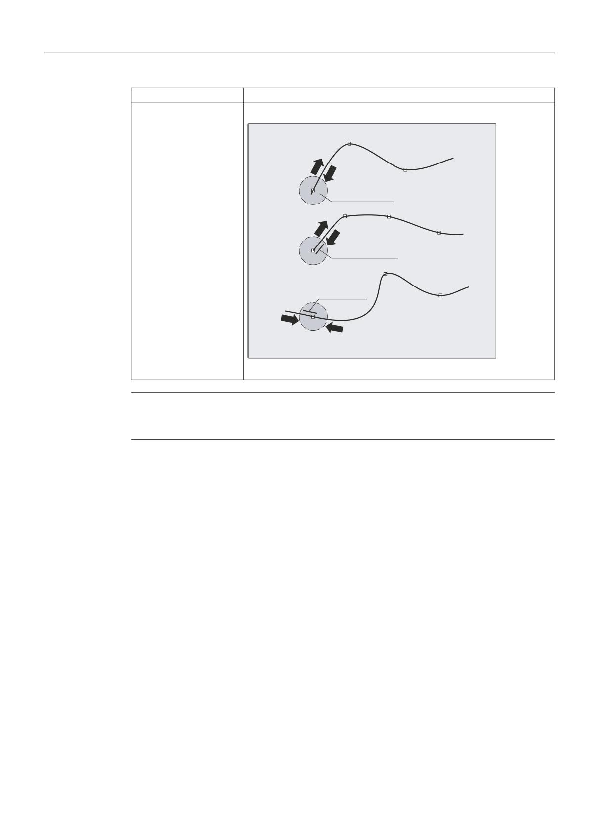
ETAN:
Tangential transition to the previous block (delete position)
%$872
($872
1R LQSXW
%1$7
(1$7
=HUR FXUYDWXUH
7DQJHQWLDO
WUDQVLWLRQ
%7$1
(7$1
Note
The programmable transitional behavior has no influence on the B spline. The B spline is
always tangential to the check polygon at its start and end points.
Supplementary conditions
● Tool radius compensation may be used.
● Collision monitoring is carried out in the projection in the plane.
Examples
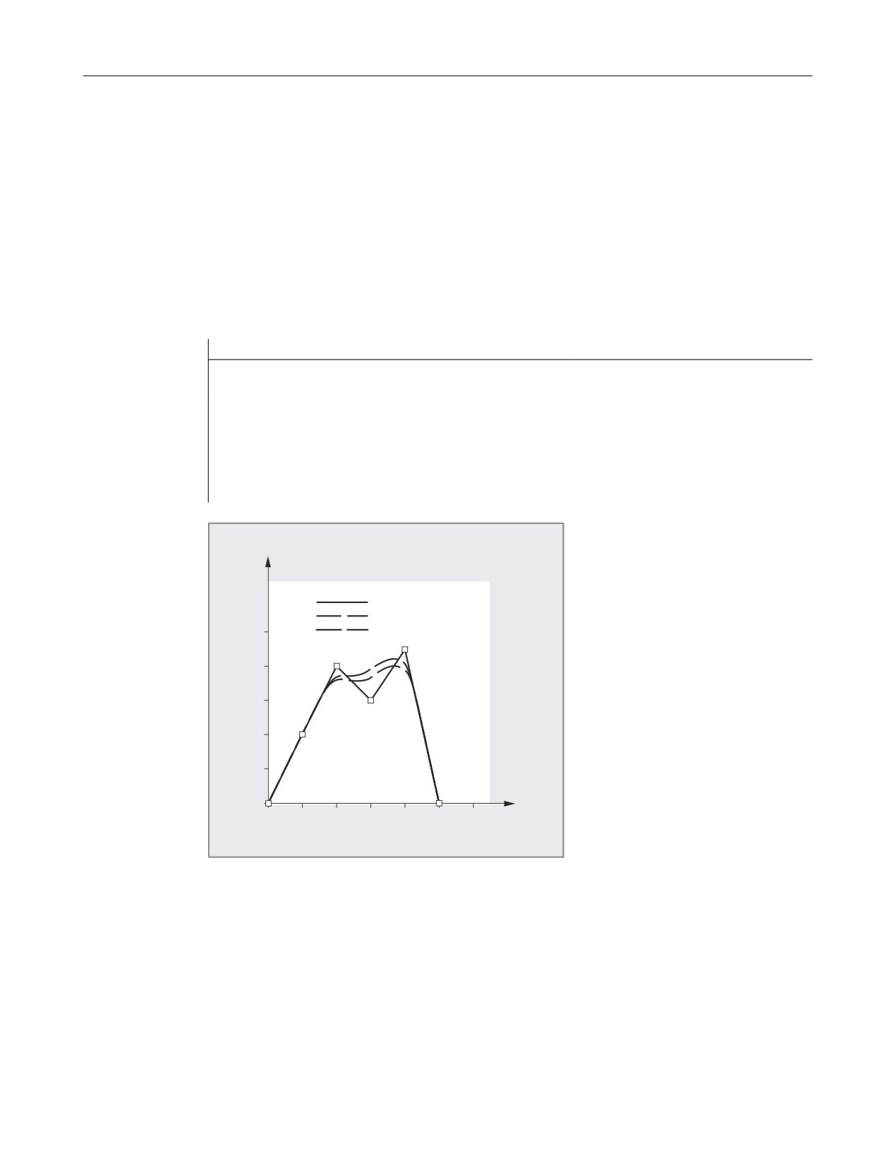
Example 1: B spline
Program code 1 (all weights 1)
N10 G1 X0 Y0 F300 G64
N20 BSPLINE
N30 X10 Y20
N40 X20 Y40
N50 X30 Y30
N60 X40 Y45
N70 X50 Y0
Job Planning
246
Programming Manual, 12/2018, A5E40869460B AB
Special motion commands
5.2 Spline interpolation (ASPLINE, BSPLINE, CSPLINE, BAUTO, BNAT, BTAN, EAUTO, ENAT, ETAN, PW, SD,
PL)
Program code 2 (different weights)
N10 G1 X0 Y0 F300 G64
N20 BSPLINE
N30 X10 Y20 PW=2
N40 X20 Y40
N50 X30 Y30 PW=0.5
N60 X40 Y45
N70 X50 Y0
Program code 3 (check polygon)
Comment
N10 G1 X0 Y0 F300 G64
N20
; n.a.
N30 X10 Y20
N40 X20 Y40
N50 X30 Y30
N60 X40 Y45
N70 X50 Y0
<
&KHFN SRO\JRQ
$OO ZHLJKWV
'LIIHUHQW ZHLJKWV
;
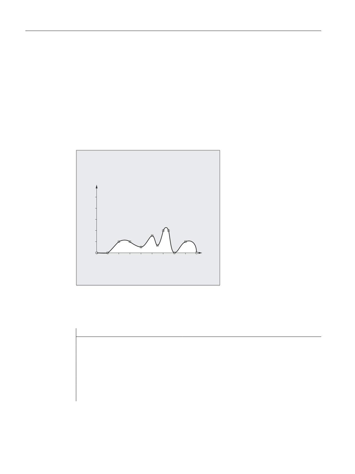
Example 2: C spline, zero curvature at the start and at the end
Program code
N10 G1 X0 Y0 F300
N15 X10
N20 BNAT ENAT
N30 CSPLINE X20 Y10
Job Planning
Programming Manual, 12/2018, A5E40869460B AB
247
Special motion commands
5.2 Spline interpolation (ASPLINE, BSPLINE, CSPLINE, BAUTO, BNAT, BTAN, EAUTO, ENAT, ETAN, PW, SD,
PL)
Program code
N40 X30
N50 X40 Y5
N60 X50 Y15
N70 X55 Y7
N80 X60 Y20
N90 X65 Y20
N100 X70 Y0
N110 X80 Y10
N120 X90 Y0
N130 M30
<
;
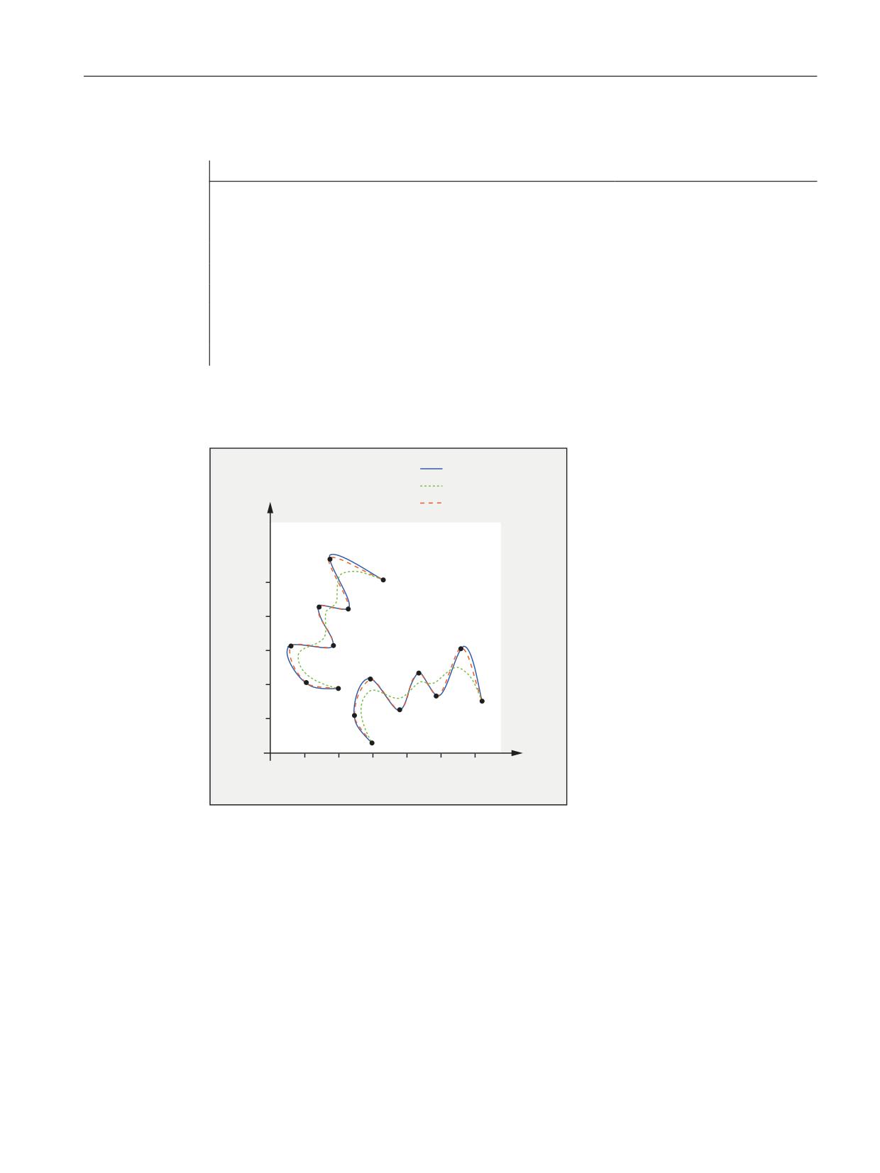
Example 3: Spline interpolation (A spline) and coordinate transformation (ROT)
Main program:
Program code
Comment
N10 G00 X20 Y18 F300 G64
; Approach starting point.
N20 ASPLINE
; Activate interpolation type A spline.
N30 CONTOUR
; First subprogram call.
N40 ROT Z-45
; Coordinate transformation: Rotation of the
WCS through -45° around the Z axis.
N50 G00 X20 Y18
; Approach contour starting point.
N60 CONTOUR
; Second subprogram call.
N70 M30
; End of program
Job Planning
248
Programming Manual, 12/2018, A5E40869460B AB
Special motion commands
5.2 Spline interpolation (ASPLINE, BSPLINE, CSPLINE, BAUTO, BNAT, BTAN, EAUTO, ENAT, ETAN, PW, SD,
PL)
Subprogram "contour" (includes the coordinates of the points along the curve):
Program code
N10 X20 Y18
N20 X10 Y21
N30 X6 Y31
N40 X18 Y31
N50 X13 Y43
N60 X22 Y42
N70 X16 Y58
N80 X33 Y51
N90 M1
In addition to the spline curve, resulting from the example program (ASPLINE), the following
diagram also contains the spline curves that would have been obtained when activating either
B or C spline interpolation (BSPLINE, CSPLINE):
$63/,1(
%63/,1(
<
&63/,1(
1
)LUVW VXESURJUDP FDOO
1
6HFRQG VXE
SURJUDP FDOO
;
Further information
Advantages of spline interpolation
With spline interpolation, the following advantages can be obtained contrary to using straight
line blocks G01:
● The number of part program blocks required to describe the contour are reduced
● Soft, curve characteristics that reduce the stress on the mechanical system at transitions
between part program blocks.
Job Planning
Programming Manual, 12/2018, A5E40869460B AB
249
Special motion commands
5.2 Spline interpolation (ASPLINE, BSPLINE, CSPLINE, BAUTO, BNAT, BTAN, EAUTO, ENAT, ETAN, PW, SD,
PL)
Properties and use of the various spline types
Spline type
Properties and use
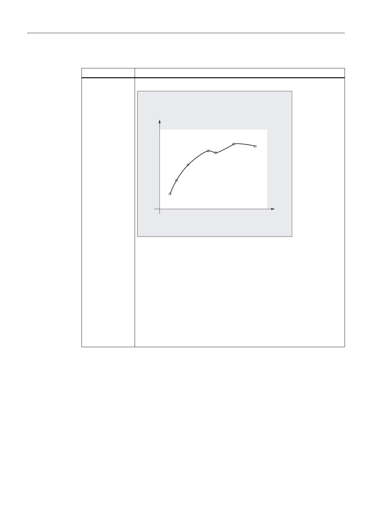
A spline
$ VSOLQH DNLPD VSOLQH
3
3
3
3
3
3
3
3
WR 3
VSHFLILHG FRRUGLQDWHV
Properties:
● Passes exactly through the specified intermediate points along the curve.
● The curve characteristic is tangential, but does not have continuous curvature.
● Produces hardly any undesirable oscillations.
● The area of influence of changes to intermediate points along the curve is
local. This means that a change to an intermediate point along the curve only
affects up to max. 6 adjacent intermediate points.
Application:
The A spline is especially suitable for interpolating curves with large changes in
the gradient (e.g. staircase-type curves and characteristics).
Job Planning
250
Programming Manual, 12/2018, A5E40869460B AB
Special motion commands
5.2 Spline interpolation (ASPLINE, BSPLINE, CSPLINE, BAUTO, BNAT, BTAN, EAUTO, ENAT, ETAN, PW, SD,
PL)
Spline type
Properties and use
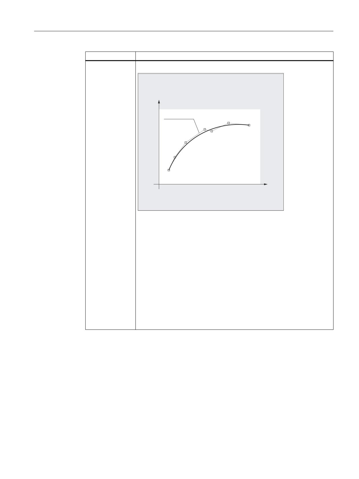
B spline
% VSOLQH
&KHFN SRO\JRQ
3
3
3
3
3
3
3
3
WR 3
VSHFLILHG FRRUGLQDWHV
Properties:
● Does not run through the specified intermediate points along the curve, but
only close to them. The intermediate points to not attract the curve. The curve
characteristic can be additionally influenced by weighting the intermediate
points using a factor.
● The curve characteristic is tangential with continuous curvature.
● Does not generate any undesirable oscillations.
● The area of influence of changes to intermediate points along the curve is
local. This means that a change to an intermediate point along the curve only
affects up to max. 6 adjacent intermediate points.
Application:
Their B spline is primarily intended as interface to CAD systems.
Job Planning
Programming Manual, 12/2018, A5E40869460B AB
251
Special motion commands
5.2 Spline interpolation (ASPLINE, BSPLINE, CSPLINE, BAUTO, BNAT, BTAN, EAUTO, ENAT, ETAN, PW, SD,
PL)
Spline type
Properties and use
C spline
& VSOLQH FXELF VSOLQH
3
3
3
3
3
3
3
3
WR 3
VSHFLILHG FRRUGLQDWHV
Properties:
● Passes exactly through the specified intermediate points along the curve.
● The curve characteristic is tangential with continuous curvature.
● Frequently generates undesirable oscillations, especially at positions where
the gradient changes significantly.
● The area of influence of changes to the intermediate points is global. This
means that if an intermediate point is changed then this influences the
complete curved characteristic.
Application:
The C spline can be well used when the intermediate points lie on a curve defined
analytically (circle, parabola, hyperbola).
Job Planning
252
Programming Manual, 12/2018, A5E40869460B AB
Special motion commands
5.2 Spline interpolation (ASPLINE, BSPLINE, CSPLINE, BAUTO, BNAT, BTAN, EAUTO, ENAT, ETAN, PW, SD,
PL)
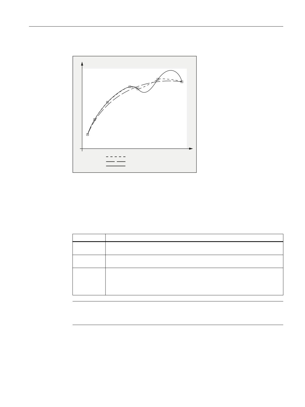
Comparison of three spline types with identical interpolation points
3
3
3
3
3
3
3
$ VSOLQH
% VSOLQH
& VSOLQH
Minimum number of spline blocks
The G codes ASPLINE, BSPLINE and CSPLINE link block end points with splines. For this
purpose, a series of blocks (end points) must be simultaneously calculated. The buffer size
for calculations is ten blocks as standard. Not every piece of block information is a spline end
point. However, the control needs a certain number of spline end-point blocks for every ten
blocks:
Spline type
Minimum number of spline blocks
A spline:
At least 4 blocks out of every 10 must be spline blocks.
These do not include comment blocks or parameter calculations.
B spline:
At least 6 blocks out of every 10 must be spline blocks.
These do not include comment blocks or parameter calculations.
C spline:
The required minimum number of spline blocks is the result of the following sum:
Value of MD20160 $MC_CUBIC_SPLINE_BLOCKS + 1
The number of points to calculate the spline segment is entered in MD20160. The
default setting is 8%. At least 9 blocks out of every 10 must be spline blocks.
Note
An alarm is output if the tolerated value is undershot and likewise when one of the axes involved
in the spline is programmed as a positioning axis.
Job Planning
Programming Manual, 12/2018, A5E40869460B AB
253
Special motion commands
5.2 Spline interpolation (ASPLINE, BSPLINE, CSPLINE, BAUTO, BNAT, BTAN, EAUTO, ENAT, ETAN, PW, SD,
PL)
Combine short spline blocks
Spline interpolation can result in short spline blocks, which reduce the path velocity
unnecessarily. The "Combine short spline blocks" function allows you to combine these blocks
such that the resulting block length is sufficient and does not reduce the path velocity.
The function is activated via the channel-specific machine data:
MD20488 $MC_SPLINE_MODE (setting for spline interpolation).
References:
Function Manual, Basic Functions; Continuous-Path Mode, Exact Stop, Look Ahead (B1),
Chapter: Combine short spline blocks
Job Planning
254
Programming Manual, 12/2018, A5E40869460B AB
Special motion commands
5.3 Spline group (SPLINEPATH)
5.3
Spline group (SPLINEPATH)
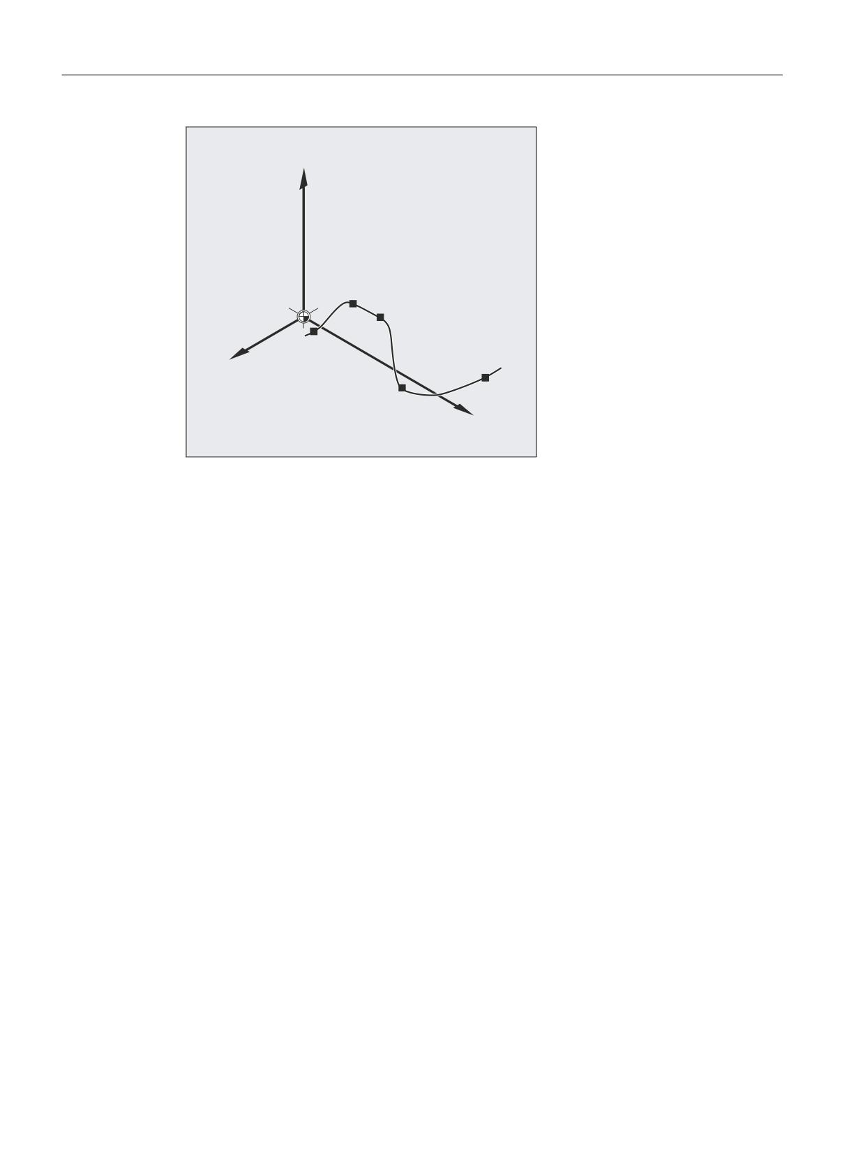
The axes to be interpolated in the spline group are selected using the SPLINEPATH command.
Up to eight path axes can be involved in a spline interpolation grouping.
Note
If SPLINEPATH is not explicitly programmed, then the first three axes of the channel are
traversed as spline group.
Syntax
The spline group is defined in a separate block:
SPLINEPATH(n,X,Y,Z,…)
Meaning
SPLINEPATH:
Command to define a spline group
n:
=1 (fixed value)
X,Y,Z,… :
Identifier of the path axes to be interpolated in the spline group
Example: Spline group with three path axes
Program code
Comment
N10 G1 X10 Y20 Z30 A40 B50 F350
N11 SPLINEPATH(1,X,Y,Z)
; Spline group
N13 CSPLINE BAUTO EAUTO X20 Y30 Z40 A50 B60
; C spline
N14 X30 Y40 Z50 A60 B70
; Intermediate points
…
N100 G1 X… Y…
; Deselect spline interpola-
tion
Job Planning
Programming Manual, 12/2018, A5E40869460B AB
255
Special motion commands
5.3 Spline group (SPLINEPATH)
=
63/,1(3$7+
;<=
;
<
Job Planning
256
Programming Manual, 12/2018, A5E40869460B AB

Special motion commands
5.4 Activating/deactivating NC block compression (COMPON, COMPCURV, COMPCAD, COMPSURF,
COMPOF)
5.4
Activating/deactivating NC block compression (COMPON,
COMPCURV, COMPCAD, COMPSURF, COMPOF)
The functions to compress linear blocks (and dependent on the parameterization, also circular
and/or rapid traverse blocks) are activated/deactivated using G commands of G group 30. The
commands are modal.
Syntax
COMPON / COMPCURV / COMPCAD / COMPSURF
COMPOF
Meaning
COMPON:
Activating the compressor function COMPON
COMPCURV:
Activating the compressor function COMPCURV
COMPCAD:
Activating the compressor function COMPCAD
COMPSURF:
Activating the compressor function COMPSURF
COMPOF :
Deactivating the currently active compressor function
Note
The rounding function G642 and jerk limitation SOFT further improve the surface quality. These
commands must be written at the beginning of the program.
Example: COMPCAD
Program code
Comment
N10 G00 X30 Y6 Z40
N20 G1 F10000 G642
; Activation: Rounding function G642
N30 SOFT
; Activation: Jerk limitation SOFT
N40 COMPCAD
; Activation: Compressor function COMPCAD
N50 STOPFIFO
N24050 Z32.499
; 1st traversing block
N24051 X41.365 Z32.500
; 2nd traversing block
N99999 X... Z...
; last traversing block
COMPOF
; compressor function off.
Job Planning
Programming Manual, 12/2018, A5E40869460B AB
257

Special motion commands
5.5 Polynomial interpolation (POLY, POLYPATH, PO, PL)
5.5
Polynomial interpolation (POLY, POLYPATH, PO, PL)
It actually involves a polynomial interpolation (POLY) and not a spline interpolation type. Its
main purpose is to act as an interface for programming externally generated spline curves
where the spline sections can be programmed directly.
This mode of interpolation relieves the NC of the task of calculating polynomial coefficients. It
can be optimally applied in cases where the coefficients are supplied directly by a CAD system
or post processor.
Syntax
3rd degree polynomial:
POLY PO[X]=(xe,a2,a3) PO[Y]=(ye,b2,b3) PO[Z]=(ze,c2,c3) PL=n
5th degree polynomial and new polynomial syntax:
POLY X=PO(xe,a2,a3,a4,a5) Y=PO(ye,b2,b3,b4,b5) Z=PO(ze,c2,c3,c4,c5)
PL=n
POLYPATH("AXES","VECT")
Note
The sum of the polynomial coefficients and axes programmed in an NC block must not exceed
the maximum permitted number of axes per block.
Meaning
POLY :
Activation of polynomial interpolation with a block
containing POLY.
POLYPATH :
Polynomial interpolation can be selected for both
AXIS or VECT axis groups
PO[axis identifier/variable] :
End points and polynomial coefficients
X, Y, Z:
Axis identifier
xe, ye, ze :
Specification of end position for the particular axis;
value range as for path dimension
a2, a3, a4, a5 :
The coefficients a2, a3, a4, and a5 are written with
their value; value range as for path dimension. The
last coefficient in each case can be omitted if it
equals zero.
PL :
Length of the parameter interval where polynomials
are defined (definition range of the function f(p)).
The interval always starts at 0, p can assume val-
ues from 0 to PL.
Theoretical value range for PL:
0.0001 … 99 999.9999
Note:
The PL value applies to the block in which it is lo-
cated. If no PL is programmed, then PL=1 is ap-
plied.
Job Planning
258
Programming Manual, 12/2018, A5E40869460B AB
Special motion commands
5.5 Polynomial interpolation (POLY, POLYPATH, PO, PL)
Activating/deactivating polynomial interpolation
The polynomial interpolation is activated in the part program using the POLX G command.
The POLY G command together with G0, G1, G2, G3, ASPLINE, BSPLINE and CSPLINE
belong to the 1st group.
Axes, which are only programmed with name and end point (e.g. X10), are linearly moved. If
all axes of an NC block are programmed in this way, the control behaves the same as for G1.
The polynomial interpolation is implicitly deactivated again by programming another command
of the 1st G group G0, G1).
Polynomial coefficient
The PO value (PO[]=) or ...=PO(...) specifies all polynomial coefficients for an axis.
Several values are specified, separated by commas corresponding the degree of the
polynomial. Different degrees of polynomials are possible for various axes within one block.
POLYPATH subprogram
Using POLYPATH(...), the polynomial interpolation can be selectively released for certain axis
groups:
Only path axes and supplementary axes:
POLYPATH("AXES")
Only orientation axes:
POLYPATH("VECT")
(when moving with orientation transformation)
The axes that are not released are linearly moved.
Polynomial interpolation is enabled as standard for both axis groups.
Polynomial interpolation is deactivated for all axes by programming without the
POLYPATH( ) parameter.
Example
Program code
Comment
N10 G1 X… Y… Z… F600
N11 POLY PO[X]=(1,2.5,0.7) PO[Y]=(0.3,1,3.2)
; Polynomial interpolation on
PL=1.5
N12 PO[X]=(0,2.5,1.7) PO[Y]=(2.3,1.7) PL=3
N20 M8 H126 …
N25 X70 PO[Y]=(9.3,1,7.67) PL=5
; Mixed data for the axes
N27 PO[X]=(10,2.5) PO[Y]=(2.3)
; No PL programmed; PL=1 applies
N30 G1 X… Y… Z.
; Polynomial interpolation off
…
Job Planning
Programming Manual, 12/2018, A5E40869460B AB
259
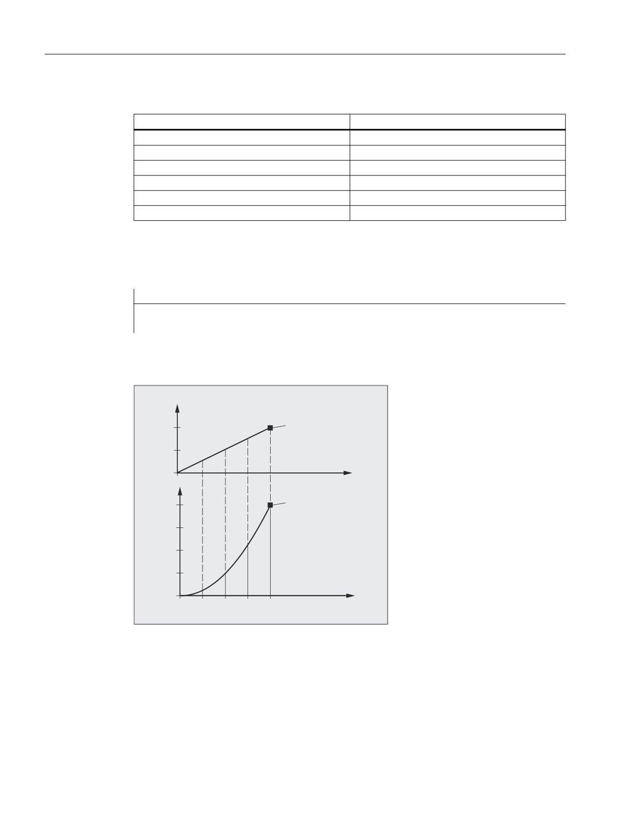
Special motion commands
5.5 Polynomial interpolation (POLY, POLYPATH, PO, PL)
Example: New polynomial syntax
Polynomial syntax that is still valid
New polynomial syntax
PO[axis identifier]=(.. , ..)
Axis identifier=PO(.. , ..)
PO[PHI]=(.. , ..)
PHI=PO(.. , ..)
PO[PSI]=(.. , ..)
PSI=PO(.. , ..)
PO[THT]=(.. , ..)
THT=PO(.. , ..)
PO[]=(.. , ..)
PO(.. , ..)
PO[variable]=IC(.. , ..)
variable=PO IC(.. , ..)
Example: Curve in the X/Y plane.
Programming
Program code
N9 X0 Y0 G90 F100
N10 POLY PO[Y]=(2) PO[X]=(4,0.25) PL=4
Shape of the curves X(p) and Y(p)
<
(QG SRLQW
S
;
(QG SRLQW
([DPSOH
1 ; < *
1
32/< 32><@
32>;@
3/
S
3/
Shape of the curve in the XY plane
Job Planning
260
Programming Manual, 12/2018, A5E40869460B AB
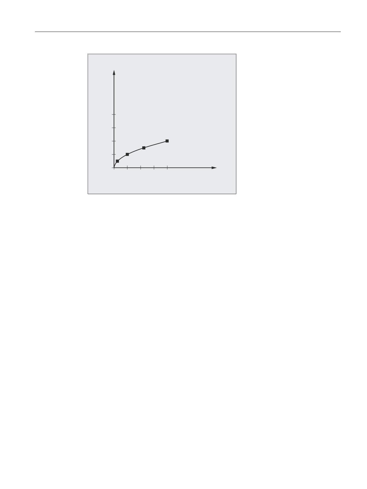
Special motion commands
5.5 Polynomial interpolation (POLY, POLYPATH, PO, PL)
<
5HVXOW LQ ;< SODQH
3/
;
Description
The equation to express the polynomial function is generally as follows:
f(p)= a0 + a1p + a2p2 + . . . + anpn
with: ai: constant coefficients (i = 0, 1, ..., n)
p: Parameter
In the control, polynomials up to a maximum of the 5th degree can be programmed:
f(p)= a0 + a1p + a2p2 + a3p3 + a4p4 + a5p5
By assigning concrete values to these coefficients, it is possible to generate various curve
shapes such as line, parabola and power functions.
A straight line is generated with a2 = a3 = a4 = a5 = 0:
f(p) = a0 + a1p
The following still applies:
a0: Axis position at the end of the preceding block
p = PL
a1 = (xE - a0 - a2*p2 - a3*p3)/p
It is possible to program polynomials without the polynomial interpolation having been activated
using the G command POLY. In this case, the programmed polynomials are not interpolated,
but instead, all of the programmed end points of the axis are linearly approached (G1). The
programmed polynomials are only moved as such after explicitly activating polynomial
interpolation in the part program (POLY).
Job Planning
Programming Manual, 12/2018, A5E40869460B AB
261
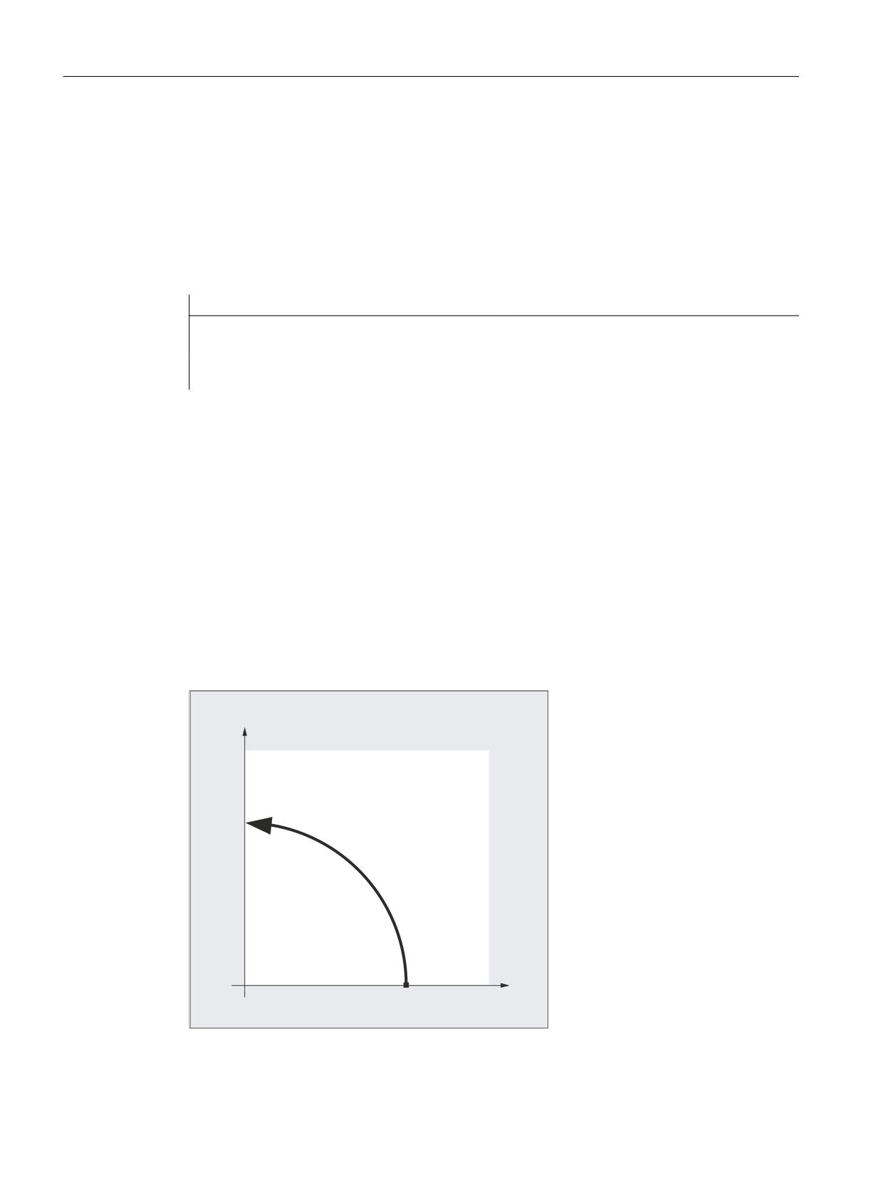
Special motion commands
5.5 Polynomial interpolation (POLY, POLYPATH, PO, PL)
Special feature: Denominator polynomial
Command PO[]=(…) can be used to program a common denominator polynomial for the
geometry axes (without specifying an axis name), i.e. the motion of the geometry axes is then
interpolated as the quotient of two polynomials.
With this programming option, it is possible to represent shapes such as conics (circle, ellipse,
parabola, hyperbola) exactly.
Example:
Program code
Comment
POLY G90 X10 Y0 F100
; Geometry axes traverse linearly to po-
sition X10 Y0.
PO[X]=(0,-10) PO[Y]=(10) PO[]=(2,1)
; Geometry axes traverse along the quad-
rant to X0 Y10.
The constant coefficient (a0) of the denominator polynomial is always assumed to be 1. The
programmed end point is independent of G90 / G91.
X(p) and Y(p) are calculated as follows from the programmed values:
X(p) = (10 - 10 * p2) / (1 + p2)
Y(p) = 20 * p / (1 + p2)
with 0 ≤ p ≤ 1
As a result of the programmed start points, end points, coefficient a2 and PL=1, the intermediate
results are as follows:
Numerator (X) = 10 + 0 * p - 10 * p2
Numerator (Y) = 0 + 20 * p + 0 * p2
Denominator =
1 + p2
<
;
Job Planning
262
Programming Manual, 12/2018, A5E40869460B AB
Special motion commands
5.5 Polynomial interpolation (POLY, POLYPATH, PO, PL)
If polynomial interpolation is active and a denominator polynomial is programmed with zeros
within the interval [0,PL], this is rejected and an alarm is output. Denominator polynomials
have no effect on the motion of special axes.
Note
Tool radius compensation can be activated with G41, G42 in conjunction with polynomial
interpolation and can be applied in the same way as in linear or circular interpolation modes.
Job Planning
Programming Manual, 12/2018, A5E40869460B AB
263

Special motion commands
5.6 Settable path reference (SPATH, UPATH)
5.6
Settable path reference (SPATH, UPATH)
For polynomial interpolation (POLY, ASPLINE, BSPLINE, CSPLINE, COMPON, COMPCURV), the
positions of the path axes i are specified as polynomials pi(U). The curve parameter U moves
from 0 to 1 within an NC block.
FGROUP selects the axes (FGROUP axes) to which the path feedrate F applies. An interpolation
with constant speed on the path S of the FGROUP axes means during the polynomial
interpolation normally a non-constant change of the curve parameter U. Consequently, two
possibilities are available for selecting the axes not contained in FGROUP on how they should
follow the FGROUP axes:
● Synchronous to path S (SPATH)
● Synchronous to curve parameter U (UPATH)
Syntax
SPATH
UPATH
Meaning
SPATH:
The axes not contained in FGROUP are traversed with reference to path S
UPATH:
The axes not contained in FGROUP are traversed with reference to curve parameter U
Note
UPATH and SPATH also define the interrelationship of the F word polynomial (FPOLY, FCUB,
FLIN) with path motion.
Supplementary conditions
SPATH and UPATH have no meaning for:
● Linear interpolation (G1)
● Circuit interpolation (G2, G3)
● Thread blocks (G33, G34, G35, G33x, G63)
● All path axes are contained in FGROUP
Example
The following example shows the difference between both types of motion control.
Program code
N10 FGROUP(X,Y,Z)
N15 G1 X0 A0 F1000 SPATH
; SPATH
N20 POLY PO[X]=(10,10) A10
Job Planning
264
Programming Manual, 12/2018, A5E40869460B AB
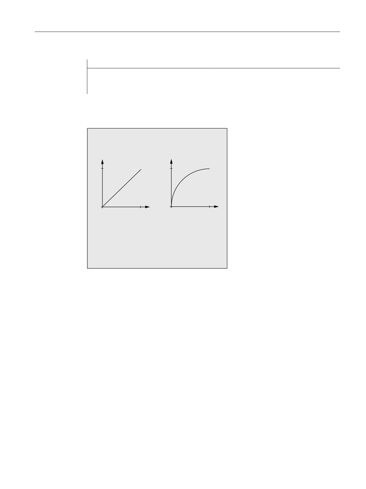
Special motion commands
5.6 Settable path reference (SPATH, UPATH)
Program code
N10 FGROUP(X,Y,Z)
N15 G1 X0 A0 F1000 UPATH
; UPATH
N20 POLY PO[X]=(10,10) A10
In both program sections, the path S of the FGROUP axes in N20 is dependent on the square
of curve parameter U. Therefore, different position arise for synchronized axis A along path X,
according to whether SPATH or UPATH is active.
63$7+
83$7+
$
$
$;
;
$;
6457 ;
;
;
'LIIHUHQW JHRPHWULFDO UHODWLRQVKLSV EHWZHHQ
D[HV IRU 63$7+ DQG 83$7+
Further information
Control behavior for reset and machine/option data
The G command, defined with MD20150 $MC_GCODE_RESET_VALUES[44], is effective
after a reset (45th. G group).
The initial state for the type of smoothing is defined with
MD20150 $MC_GCODE_RESET_VALUES[9] (10th G group).
The axis-specific machine data MD33100 $MA_COMPRESS_POS_TOL[<n>] has an
extended significance: It contains the tolerances for the compressor function and for smoothing
with G642.
Job Planning
Programming Manual, 12/2018, A5E40869460B AB
265
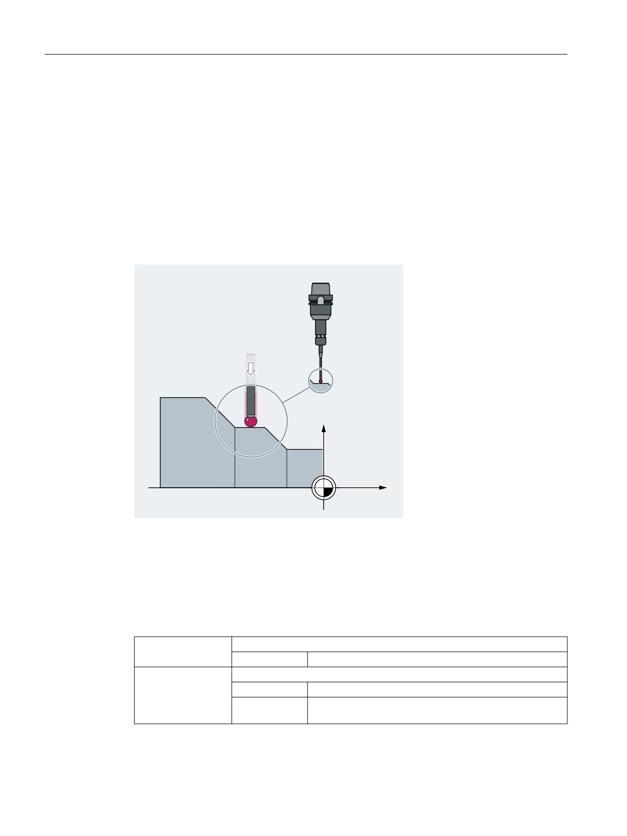
Special motion commands
5.7 Channel-specific measuring (MEAS, MEAW)
5.7
Channel-specific measuring (MEAS, MEAW)
In the case of channel-specific measuring, the measuring process for an NC channel is always
activated from the part program running in the relevant channel. One trigger event (positive or
negative edge of the probe) and one measuring mode with deletion of distance-to-go (MEAS)
or without deletion of distance-to-go (MEAW) are programmed in a measuring block. All the
axes programmed in the measuring block then take part in the measuring process.
As soon as a measuring block becomes active, the probe is moved to the workpiece. On the
probe's switching edge, the positions for all axes programmed in the measuring block are
measured and written to the appropriate memory cell for each axis.
The results of measurements can be read in the part program or with synchronized actions in
both the machine and the workpiece coordinate systems.
;
=
Syntax
MEAS=<TE> G... X... Y... Z...
MEAW=<TE> G... X... Y... Z...
Meaning
MEAS:
Measurement with delete distance-to-go
Effectiveness:
Non-modal
MEAW:
Measurement without delete distance-to-go
Effectiveness:
Non-modal
Application:
For measuring tasks in which the programmed position is to
be approached in every case.
Job Planning
266
Programming Manual, 12/2018, A5E40869460B AB
Special motion commands
5.7 Channel-specific measuring (MEAS, MEAW)
<TE>:
Trigger event to initiate measurement
Type:
INT
Range of val-
-2, -1, 1, 2
ues:
Value:
(+)1
Positive edge of probe 1 (on measuring input 1)
-1
Negative edge of probe 1 (on measuring input 1)
(+)2
Positive edge of probe 2 (on measuring input 2)
-2
Negative edge of probe 2 (on measuring input 2)
Note:
There is a maximum of 2 probes (dependent on configuration level).
G...:
Type of interpolation, e.g. G0, G1, G2 or G3
X... Y... Z...:
End points in Cartesian coordinates
Note
MEAS and MEAW are non-modal, and programmed together with motion operations. The
feedrate and interpolation type (G0, G1, etc.) as well as the number of axes must be adapted
for the respective measuring task.
Example
Program code
Comment
N10 MEAS=1 G1 F1000 X100 Y730 Z40
; Measuring block with probe at first
measuring input and linear interpola-
tion. A preprocessing stop is automati-
cally generated.
Further information
Query status
If an evaluation is required in the program, whether a probe has been deflected or has switched,
the status can be queried through the following system variables:
System variable
Meaning
Data type
Value
$A_PROBE[<n>]
Probe state
INT
0
Probe not deflected.
1
Probe deflected.
$AC_MEA[<n>]
Switching status of the probe
INT
0
Probe has not switch-
ed
$AC_MEA[<n>] is automati-
cally reset at the beginning of
1
Probe has switched.
a measurement.
<n> = number of the probe
Job Planning
Programming Manual, 12/2018, A5E40869460B AB
267

Special motion commands
5.7 Channel-specific measuring (MEAS, MEAW)
Reading measured values
For channel-specific measuring, the positions of all traversing path and positioning axes of the
block are acquired (maximum number of axes depends on the control configuration). For
MEAS, the motion is braked in a defined fashion after the probe has been triggered.
Note
If a geometry axis is programmed in a measuring block, the measured values are stored for
all current geometry axes.
If an axis participating in a transformation is programmed in a measuring block, the measured
values are stored for all axes participating in this transformation.
Reading measurement results
The measured values of the axes acquired by probes can be read through the following system
variables in the part program and in synchronized actions.
System variable
Meaning
$AA_MM[<Axis>]
Probe measured value in the machine coordinate system
$AA_MW[<Axis>]
Probe measured value in the workpiece coordinate system
Job Planning
268
Programming Manual, 12/2018, A5E40869460B AB

Special motion commands
5.8 Axis-specific measurement (MEASA, MEAWA, MEAC) (option)
5.8
Axis-specific measurement (MEASA, MEAWA, MEAC) (option)
With axis-specific measuring, activation can take place in the part program or in synchronized
actions. If two measuring systems are available for the axis, both can be used for the
measurement.
The following measuring methods are available:
● Measurement with delete distance-to-go (MEASA)
● Measurement without delete distance-to-go (MEAWA)
● Continuous measurement without delete distance-to-go (MEAC)
With MEASA or MEAWA for the programmed axis, up to four measured values are acquired
for each measurement and are then saved in system variables in accordance with the trigger
event.
With continuous measurement with MEAC, the measurement results are stored in FIFO
variables.
Syntax
MEASA[<Axis>]=(<Mode>,<TE1>,...,<TE4>)
MEAWA[<Axis>]=(<Mode>,<TE1>,...,<TE4>)
MEAC[<Axis>]=(<Mode>,<MeasMem>,<TE1>,...,<TE4>)
Note
MEASA and MEAWA are non-modal; and can be programmed together in one block. If, on
the contrary, MEASA/MEAWA are programmed with MEAS/MEAW in one block, there is an
error message.
Meaning
MEASA:
Axis-specific measurement with deletion of distance-to-go
Effectiveness:
Non-modal
MEAWA:
Axes-specific measurement without delete distance-to-go
Effectiveness:
Non-modal
MEAC:
Axis-specific, continuous measurement without delete distance-to-go
Effectiveness:
Non-modal
<Axis>:
Name of channel axis used for measurement
Job Planning
Programming Manual, 12/2018, A5E40869460B AB
269
Special motion commands
5.8 Axis-specific measurement (MEASA, MEAWA, MEAC) (option)
<Mode>:
Two-digit (xx) number indicating the operating mode (measuring mode and meas-
uring system)
Units decade: Measuring mode
Specifies whether the trigger events are to be activated in chronological or pro-
grammed order.
x0
Cancel measuring job.
x1
Up to 4 different trigger events can be activated simultaneously.
x2
Up to 4 trigger events that can be activated successively.
x3
Up to 4 different trigger events can be activated in succession, but there
is no monitoring of trigger event 1 at the start (alarms 21700/21703 are
suppressed).
Note:
MEAC does not support this mode.
Tens decade: Measuring system
Specifies the measuring system with which measuring is to be performed.
0x (or no specification)
Active measuring system
1x
Measuring system 1
2x
Measuring system 2
3x
Both measuring systems
<TE>:
Trigger event to initiate measurement
Type:
INT
Range of val-
-2, -1, 1, 2
ues:
(+)1
Positive edge of probe 1
-1
Negative edge of probe 1
(+)2
Positive edge of probe 2
-2
Negative edge of probe 2
Note:
If the measuring process is performed with two measuring systems, a maximum
of two trigger events can be programmed (positive or negative edge). The meas-
ured values of both measuring systems are acquired for both the trigger events.
<MeasMem>:
Number of FIFO (circular buffer)
Examples
Example 1: Axis-specific measurement with delete distance-to-go in mode 1 (evaluation in
chronological sequence)
a) Measuring with one measuring system
Program code
Comment
N100 MEASA[X]=(1,1,-1) G01 X100 F100
; Measuring in mode 1 with active measur-
ing system. Wait for measuring signal
with positive/negative edge from probe 1
for travel path to X=100.
N110 IF $AC_MEA[1]==FALSE GOTOF END
; Check that the measurement was success-
ful.
Job Planning
270
Programming Manual, 12/2018, A5E40869460B AB
Special motion commands
5.8 Axis-specific measurement (MEASA, MEAWA, MEAC) (option)
Program code
Comment
N120 R10=$AA_MM1[X]
; Save measured value acquired at the
first programmed trigger event (positive
edge).
N130 R11=$AA_MM2[X]
; Save measured value acquired at the sec-
ond programmed trigger event (negative
edge).
N140 END:
b) Measuring with two measuring systems
Program code
Comment
N200 MEASA[X]=(31,1,-1) G01 X100 F100
; Measuring in mode 1 with both measuring
systems. Wait for measuring signal with
positive/negative edge from probe 1 for
travel path to X=100.
N210 IF $AC_MEA[1]==FALSE GOTOF END
; Check that the measurement was success-
ful.
N220 R10=$AA_MM1[X]
; Save measured value of measuring system
1 at positive edge.
N230 R11=$AA_MM2[X]
; Save measured value of measuring system
2 at positive edge.
N240 R12=$AA_MM3[X]
; Save measured value of measuring system
1 at negative edge.
N250 R13=$AA_MM4[X]
; Save measured value of measuring system
2 at negative edge.
N260 END:
Example 2: Axis-specific measurement with delete distance-to-go in mode 2 (evaluation in
programmed sequence)
Program code
Comment
N100 MEASA[X]=(2,1,-1,2,-2) G01 X100 F100
; Measuring in mode 2 with active measur-
ing system. Wait for measuring signal in
the sequence positive edge probe 1, nega-
tive edge probe 1, positive edge probe 2,
negative edge probe 2 while traversing
path to X=100.
N110 IF $AC_MEA[1]==FALSE GOTOF PROBE2
; Check that the measurement with probe 1
is successful.
N120 R10=$AA_MM1[X]
; Save measured value acquired at the
first programmed trigger event (positive
edge of probe 1).
N130 R11=$AA_MM2[X]
; Save measured value acquired at the sec-
ond programmed trigger event (positive
edge of probe 1).
N140, PROBE2:
Job Planning
Programming Manual, 12/2018, A5E40869460B AB
271
Special motion commands
5.8 Axis-specific measurement (MEASA, MEAWA, MEAC) (option)
Program code
Comment
N150 IF $AC_MEA[2]==FALSE GOTOF END
; Check that the measurement with probe 2
is successful.
N160 R12=$AA_MM3[X]
; Save measured value acquired at the
third programmed trigger event (positive
edge of probe 2).
N170 R13=$AA_MM4[X]
; Save measured value acquired at the
fourth programmed trigger event (positive
edge of probe 2).
N180 END:
Example 3: Axis-specific, continuous measurement in mode 1 (evaluation in chronological
sequence)
a) Measurement of up to 100 measured values
Program code
Comment
N110 DEF REAL MEASVALUE[100]
N120 DEF INT loop=0
N130 MEAC[X]=(1,1,-1) G01 X1000 F100
; Measuring in mode 1 with active measur-
ing system, save measured values under
$AC_FIFO1, wait for measuring system with
negative edge from probe 1 on the travel
path to X=1000.
N135 STOPRE
N140 MEAC[X]=(0)
; Terminate measurement when axis posi-
tion is reached.
N150 R1=$AC_FIFO1[4]
; Save number of accumulated measured val-
ues in parameter R1.
N160 FOR loop=0 TO R1-1
N170 MEASURED VALUE[loop]=$AC_FIFO1[0]
; Read-out measured values from $AC_FIFO1
and save.
N180 ENDFOR
b) Measurement with delete distance-to-go after 10 measured values
Program code
Comment
N10 WHEN $AC_FIFO1[4]>=10 DO MEAC[x]=(0) DELDTG(x)
; Delete distance-to-go.
N20 MEAC[x]=(1,1,1,-1) G01 X100 F500
N30 MEAC [X]=(0)
N40 R1 = $AC_FIFO1[4]
; Number of measured values.
Job Planning
272
Programming Manual, 12/2018, A5E40869460B AB
Special motion commands
5.8 Axis-specific measurement (MEASA, MEAWA, MEAC) (option)
c) Measurement of a positive/negative tooth flank with 2 probes
Program code
Comment
N110 DEF REAL MEASVALUE[16]
N120 DEF INT loop=0
N130 MEAC[X]=(1,1,-1,2) G01 X100 F100
; Measurement in mode 1 with active meas-
uring system, save measured values under
$AC_FIFO1, wait for measuring signal in
the sequence negative edge of probe 1,
positive edge of probe 2 while traversing
the travel path to X=100.
N140 STOPRE
; Preprocessing stop.
N150 MEAC[X]=(0)
; Terminate measurement when axis posi-
tion is reached.
N160 R1=$AC_FIFO1[4]
; Save number of accumulated measured val-
ues in parameter R1.
N170 FOR loop=0 TO R1-1
N180 MEASURED VALUE[loop]=$AC_FIFO1[0]
; Read-out measured values from $AC_FIFO1
and save.
N190 ENDFOR
Further information
Measuring job
A measuring job can be programmed in the part program or from a synchronized action. Please
note that only one measuring job can be active at any given time for each axis.
Note
The feed must be adjusted to suit the particular measuring task
In the case of MEASA and MEAWA, the correctness of results can be only guaranteed for
feedrates at which no more than one trigger event of the same type and no more than 4 trigger
events of different types occur in each position control cycle.
In the case of continuous measurement with MEAC, the ratio between interpolator cycle and
the position control cycle must not exceed 1:8.
Trigger event
A trigger event comprises the number of the probe and the trigger criterion (positive or negative
edge) of the measuring signal.
Up to 4 trigger events of the addressed probe can be processed for each measurement; in
other words, up to two probes each with two measuring signal edges. The processing
sequence and the maximum number of trigger events depend on the selected mode.
Job Planning
Programming Manual, 12/2018, A5E40869460B AB
273
Special motion commands
5.8 Axis-specific measurement (MEASA, MEAWA, MEAC) (option)
If the measuring operation is performed with two measuring systems, a maximum of two trigger
events can be programmed (positive or negative edge). The measured values of both probes
are acquired for both of the trigger events.
Note
With the use of PROFIBUS telegram 391 (default setting for PROFIBUS communication) only
one measured value is possible for each trigger event and position control cycle.
For MEAC, the number of measured values per trigger event can be increased by using
PROFIBUS telegram 395 to a total of 8 measured values for a positive edge and 8 measured
values for a negative edge for each trigger event and position control cycle:
● One probe: 8 measured values for a positive and 8 for a negative edge
● Two probes: 4 measured values for a positive and 4 for a negative edge for each probe
This means that higher feed rates or higher speeds can be reached by using PROFIBUS
telegram 395.
Operating mode
The first digit (tens decade) of the operating mode selects the required measuring system. If
only one measuring system is installed, but a second is programmed, the installed system is
automatically selected.
The second digit (units decade) selects the desired measuring mode. The measuring process
is thus adapted to the options supported by the relevant control:
● Mode 1
Trigger events are evaluated in the chronological sequence in which they occur. When this
mode is selected, only one trigger event can be programmed for six-axis modules. If more
than one trigger event is specified, the mode selection is switched automatically to mode
2 (without message).
● Mode 2
Trigger events are evaluated in the programmed sequence.
● Mode 3
Trigger events are evaluated in the programmed sequence but there is no monitoring of
trigger event 1 at the start.
Measurement with and without delete distance-to-go
When command MEASA is programmed, the distance-to-go is not deleted until all required
measured values have been acquired.
MEAWA is used for special measuring tasks in which a programmed position always has to
be approached.
Note
MEASA cannot be programmed in synchronized actions. As an alternative, MEAWA plus
delete distance-to-go can be programmed as a synchronized action.
If the measuring job with MEAWA is started from synchronized actions, the measured values
will only be available in the machine coordinate system.
Job Planning
274
Programming Manual, 12/2018, A5E40869460B AB
Special motion commands
5.8 Axis-specific measurement (MEASA, MEAWA, MEAC) (option)
Geometry axes/transformations
If axial measurement is to be started for a geometry axis, the same measuring job must be
programmed explicitly for all remaining geometry axes. The same applies to axes involved in
a transformation.
Examples:
N10 MEASA[Z]=(1,1) MEASA[Y]=(1,1) MEASA[X]=(1,1) G0 Z100
or
N10 MEASA[Z]=(1,1) POS[Z]=100
Query status
If an evaluation is required in the program, whether a probe has been deflected or has switched,
the status can be queried through the following system variables:
System variable
Meaning
Data type
Value
$A_PROBE[<n>]
Probe state
INT
0
Probe not deflected.
1
Probe deflected.
$AC_MEA[<n>]
Switching status of the probe
INT
0
Probe has not switch-
ed
$AC_MEA[<n>] is automati-
cally reset at the beginning of
1
Probe has switched
a measurement.
(all trigger events pro-
grammed in the
measuring block
have taken place).
<n> = number of the probe
Note
If measurement is started from synchronized actions, $AC_MEA is no longer updated. In this
case, the NC/PLC interface signal DB31, … DBX62.3 or the equivalent variable
$AA_MEAACT[<Axis>] must be queried.
$AA_MEAACT==1: Measurement active
$AA_MEAACT==0: Measurement not active
Probe limitation
In the NC program or synchronized action, the probe limiting status can be read using system
variable $A_PROBE_LIMITED when using PROFIBUS telegram 395:
$A_PROBE_LIMITED[<n>] == 0: Probe limitation inactive/reset
$A_PROBE_LIMITED[<n>] == 1: Probe limitation active
<n> = probe number
Job Planning
Programming Manual, 12/2018, A5E40869460B AB
275
Special motion commands
5.8 Axis-specific measurement (MEASA, MEAWA, MEAC) (option)
Measurement results for MEASA / MEAWA
The values measured by probes can be read through the following system variables in the part
program and in synchronized actions.
System variable
Meaning
$AA_MM1[<Axis>]
Probe measured value for trigger event 1 in the machine coordinate system
$AA_MM4[<Axis>]
Probe measured value for trigger event 4 in the machine coordinate system
$AA_MW1[<Axis>]
Probe measured value for trigger event 1 in the workpiece coordinate system
$AA_MW4[<Axis>]
Probe measured value for trigger event 4 in the workpiece coordinate system
<Axis> = measuring axis
If a measuring job is executed by two measuring systems, each of the two possible trigger
events is acquired from both measuring systems. The assignment of system variables is then
as follows:
$AA_MM1[<Axis>]
or
$AA_MW1[<Axis>]
Measured value from measuring sys-
tem 1 on trigger event 1
$AA_MM2[<Axis>]
or
$AA_MW2[<Axis>]
Measured value from measuring sys-
tem 2 on trigger event 1
$AA_MM3[<Axis>]
or
$AA_MW3[<Axis>]
Measured value from measuring sys-
tem 1 on trigger event 2
$AA_MM4[<Axis>]
or
$AA_MW4[<Axis>]
Measured value from measuring sys-
tem 2 on trigger event 2
Continuous measurement (MEAC)
The measured values for MEAC are available in the machine coordinate system and stored
in the programmed FIFO[<n>] memory (circular buffer). If two probes are configured for the
measurement, the measured values of the second probe are stored separately in the FIFO[<n>
+1] memory configured specifically for this purpose (defined in machine data).
The FIFO memory is a circular buffer in which measured values are written to $AC_FIFO
variables according to the circular principle.
Note
FIFO contents can be read only once from the circular buffer. If this measured data is to be
used several times, it must be buffered in the user data.
If the number of measured values for the FIFO memory exceeds the maximum value defined
in machine data, the measurement is automatically terminated.
An endless measuring process can be implemented by reading out measured values cyclically.
In this case, data must be read out at least with the same frequency as new measured values
are input.
References:
Function Manual Synchronized Actions; "Detailed description" Chapter > "Parameters
($AC_FIFO)"
Job Planning
276
Programming Manual, 12/2018, A5E40869460B AB
Special motion commands
5.8 Axis-specific measurement (MEASA, MEAWA, MEAC) (option)
Protection against programming errors
The following programming errors are detected and indicated as errors:
● MEASA/MEAWA programmed with MEAS/MEAW in the same block
Example:
N01 MEAS=1 MEASA[X]=(1,1) G01 F100 POS[X]=100
● MEASA/MEAWA with number of parameters <2 or >5
Example:
N01 MEAWA[X]=(1) G01 F100 POS[X]=100
● MEASA/MEAWA with trigger event not equal to 1/ -1/ 2/ -2
Example:
N01 MEASA[B]=(1,1,3) B100
● MEASA/MEAWA with invalid mode
Example:
N01 MEAWA[B]=(4,1) B100
● MEASA/MEAWA with trigger event programmed twice
Example:
N01 MEASA[B]=(1,1,-1,2,-1) B100
● MEASA/MEAWA and missing geometry axis
Example:
N01 MEASA[X]=(1,1) MEASA[Y]=(1,1) G01 X50 Y50 Z50 F100; GEO axis X/
Y/Z
● Inconsistent measuring job with geometry axes
Example:
N01 MEASA[X]=(1,1) MEASA[Y]=(1,1) MEASA[Z]=(1,1,2) G01 X50 Y50 Z50
F100
See also
Synchronized actions (Page 597)
Job Planning
Programming Manual, 12/2018, A5E40869460B AB
277
Special motion commands
5.9 Special functions for OEM users (OMA1 ... OMA5, OEMIPO1, OEMIPO2, G810 ... G829)
5.9
Special functions for OEM users (OMA1 ... OMA5, OEMIPO1,
OEMIPO2, G810 ... G829)
OEM addresses
The meaning of OEM addresses is determined by the OEM user. Their functionality is
incorporated by means of compile cycles. Five OEM addresses are reserved (OMA1 ... OMA5).
The address identifiers are settable. OEM addresses can be programmed in any block.
Reserved G command calls
The following G command calls are reserved for OEM users:
● OEMIPO1, OEMIPO2 (from G group 1)
● G810 ... G819 (G group 31)
● G820 ... G829 (G group 32)
Their functionality is incorporated by means of compile cycles.
Functions and subprograms
OEM users can also set up predefined functions and subprograms with parameter transfer.
Note
Workpiece simulation
Up to SW 4.4, no compile cycles were supported, as of SW 4.4, only selected compile cycles
(CC) are supported for the workpiece simulation.
Language commands in the part program of compile cycles that are not supported
(OMA1 ... OMA5, OEMIPO1/2, G810 ... G829, own procedures and functions) - therefore result
in an alarm message and cancellation of the simulation without any individual handling.
Solution: Individually handle the missing CC-specific language elements in the part program
($P_SIM query).
Example:
N1 G01 X200 F500
IF (1==$P_SIM)
N5 X300 ;not active for CC simulation
ELSE
N5 X300 OMA1=10
ENDIF
Job Planning
278
Programming Manual, 12/2018, A5E40869460B AB
Special motion commands
5.10 Feedrate reduction with corner deceleration (FENDNORM, G62, G621)
5.10
Feedrate reduction with corner deceleration (FENDNORM, G62,
G621)
With automatic corner deceleration the feed rate is reduced according to a bell-shaped curve
before reaching the corner. It is also possible to parameterize the extent of the tool behavior
relevant to machining via setting data. These are:
● Start and end of feed rate reduction
● Override with which the feed rate is reduced
● Detection of a relevant corner
Relevant corners are those whose inside angle is less than the corner parameterized in the
setting data.
Default value FENDNORM deactivates the function of the automatic corner override.
References:
/FBFA/ "Function Description ISO Dialects"
Syntax
FENDNORM
G62 G41
G621
Meaning
FENDNORM:
Automatic corner deceleration OFF
G62:
Corner deceleration at inside corners when tool radius offset is active
G621:
Corner deceleration at all corners when tool radius offset is active
G62 only applies to inside corners with
● active tool radius offset G41, G42 and
● active continuous-path mode G64, G641
The corner is approached at a reduced feed rate resulting from:
F * (override for feed rate reduction) * feed rate override
The maximum possible feed rate reduction is attained at the precise point where the tool is to
change directions at the corner, with reference to the center path.
G621 applies analogously with G62 at each corner of the axes defined by FGROUP.
Job Planning
Programming Manual, 12/2018, A5E40869460B AB
279
Special motion commands
5.11 Programmable end of motion criteria (FINEA, COARSEA, IPOENDA, IPOBRKA, ADISPOSA)
5.11
Programmable end of motion criteria (FINEA, COARSEA, IPOENDA,
IPOBRKA, ADISPOSA)
Similar to the block change criterion for path interpolation (G601, G602, and G603) it is also
possible to program the end-of-motion criterion for single-axis interpolation in a part program
or in synchronized actions for command/PLC axes.
The end-of-motion criterion set will affect how quickly or slowly part program blocks and
technology cycle blocks with single-axis movements are completed. The same applies for PLC
via FC15/16/18.
Syntax
FINEA[<axis>]
COARSEA[<axis>]
IPOENDA[<axis>]
IPOBRKA(<axis>[,<instant in time>])
ADISPOSA[<axis>]=(<mode>,<window size>)
Meaning
FINEA:
End-of-motion criterion: "Exact stop fine"
Effective:
Modal
COARSEA:
End-of-motion criterion: "Exact stop coarse"
Effective:
Modal
IPOENDA:
End-of-motion criterion: "Interpolator stop"
Effective:
Modal
IPOBRKA:
Block change criterion: Braking ramp
Effective:
Modal
ADISPOSA:
Tolerance window for end-of-motion criterion
Effective:
Modal
<axis>:
Channel axis name (X, Y,
)
<instant in time>:
Time of the block change, referred to the braking ramp as a %:
●
100% = start of the braking ramp
●
0% = end of the braking ramp, the same significance as IPOENDA
Type:
REAL
<mode>:
Reference of the tolerance window
Range of values:
0
Tolerance window not active
1
Tolerance window with respect to set posi-
tion
2
Tolerance window with respect to actual po-
sition
Type:
INT
<window size>:
Size of the tolerance window
Type:
REAL
Job Planning
280
Programming Manual, 12/2018, A5E40869460B AB
Special motion commands
5.11 Programmable end of motion criteria (FINEA, COARSEA, IPOENDA, IPOBRKA, ADISPOSA)
Examples
Example 1: End-of-motion criterion: "Interpolator stop"
Program code
; traverse positioning axis X to 100, velocity 200 m/
min, acceleration 90%,
; end-of-motion criterion: Interpolator stop
N110 G01 POS[X]=100 FA[X]=200 ACC[X]=90 IPOENDA[X]
; Synchronized action:
; ALWAYS IF: Input 1 is set
; THEN traverse positioning axis X to 50, velocity 200
m/min, acceleration 140%,
;
end-of-motion criterion: Interpolator stop
N120 EVERY $A_IN[1] DO POS[X]=50 FA[X]=200 ACC[X]=140
IPOENDA[X]
Example 2: Block change criterion: "Braking ramp"
Program code
Comment
; Default setting is effective
N40 POS[X]=100
; Positioning motion from X to position 100.
Block change criterion: Exact stop fine
N20 IPOBRKA(X,100)
; Block change criterion: "Braking ramp",
100% = start of the braking ramp
N30 POS[X]=200
; The block is changed as soon as the X axis starts to brake
N40 POS[X]=250
; X axis no longer brakes at position 200, but rather contin-
ues to traverse to position 250.
As soon as the axis starts to brake, the block changes.
N50 POS[X]=0
; Axis X brakes and returns to position 0.
The block change takes place at position 0 and "exact stop
fine"
N60 X10 F100
; Axis X traverses as path axis to position 10
Further information
System variable for end-of-motion criterion
The effective end-of-motion criterion can be read using the system variable $AA_MOTEND.
References: /LIS2sl/ List Manual, Book 2
Block-change criterion: "Braking ramp" (IPOBRKA)
If, when activating the block change criterion "brake ramp", a value is programmed for the
optional block change instant in time, then this becomes effective for the next positioning
motion and is written into the setting data synchronized to the main run. If no value is specified
for the block change instant in time, then the actual value of the setting data is effective.
Job Planning
Programming Manual, 12/2018, A5E40869460B AB
281