SINUMERIK 840D sl. Service - Functions. Manual (2018-2020) - page 100
Orientation transformations
6.5 Parameterization with machine data (conventional)
WR
W
WR
PR
W
[
PR
[
%
SR
=
%
&
PR
MR
&
;
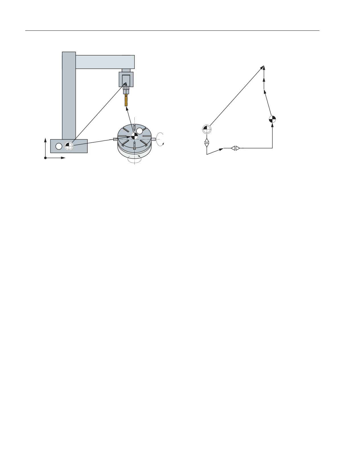
①
Machine zero
②
Zero point tool table
mo
Position vector in MCS
po
$MC_TRAFO5_PART_OFFSET_<x>[0 ..2]
x
Vector of programmed position in BCS
t
Tool correction vector
to
$MC_TRAFO5_BASE_TOOL_<x>[0 .. 2]
jo
$MC_TRAFO5_JOINT_OFFSET_<x>[0 .. 2]
Figure 6-8
Schematic diagram of CB kinematics, moved workpiece
Transformations
250
Function Manual, 10/2020, 6FC5397-5GP40-0BA1
Orientation transformations
6.5 Parameterization with machine data (conventional)
$
$
WR
W
WR
PR
[
W
PR
[
SR
=
SR
MR
&
&
;
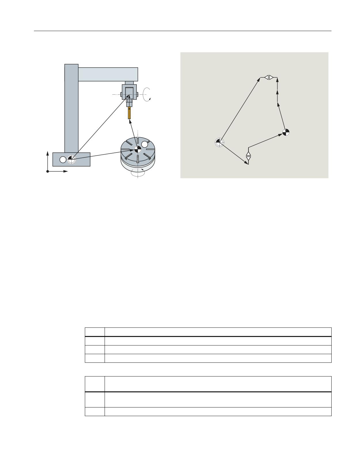
①
Machine zero
②
Zero point tool table
mo
Position vector in MCS
po
$MC_TRAFO5_PART_OFFSET_<x>[0 ..2]
x
Vector of programmed position in BCS
t
Tool correction vector
to
$MC_TRAFO5_BASE_TOOL_<x>[0 .. 2]
jo
$MC_TRAFO5_JOINT_OFFSET_<x>[0 .. 2]
Figure 6-9
Schematic diagram of AC kinematics, moved tool, moved workpiece, moved tool
Sign handling for rotary axes
The sign handling of rotary axes involved in 5-axis transformation is set in the channel using
machine data:
$MC_TRAFO5_ROT_SIGN_IS_PLUS_<x>[ <n> ] = <value>
where x = 1, 2, ... maximum number of transformations in the channel
<n>
Meaning
0
1st rotary axis
1
2nd rotary axis
2
3rd rotary axis
<Val-
Meaning
ue>
TRUE
The sign is not inverted. The traversing direction is as defined in MD32100 $MA_AX_MO-
TION_DIR.
FALSE
The sign is inverted.
Transformations
Function Manual, 10/2020, 6FC5397-5GP40-0BA1
251

Orientation transformations
6.5 Parameterization with machine data (conventional)
The machine data is not used to define that the direction of rotation of the rotary axis involved
is changed. Instead, it is specified as to whether the rotary axis, for traversing motion, rotates in
the positive traversing direction in the mathematical positive (counterclockwise) or negative
(clockwise) direction. The consequence when changing this machine data is therefore not a
change in the direction of rotation, but a change in the compensating motion in the linear axes.
However, if a direction vector, and therefore implicitly compensation motion is specified, then
the direction of rotation of the rotary axis involved changes.
This means that at a real machine, the machine data only has to be set to FALSE if, for traversing
motion in the positive traversing direction, the rotary axis rotates in the mathematical positive
direction (counterclockwise).
6.5.1.3
Activation via parts/program/softkey
The machine data relevant to the kinematic transformation has thus far been activated mostly
through POWER ON.
Transformation machine data can also be activated via the part program / softkey and it is not
necessary to boot the control system.
Additional information
Cartesian PTP travel (Page 177)
6.5.1.4
3-axis and 4-axis transformations
3 and 4-axis transformations are special types of 5-axis transformations, where the tool can only
be orientated in the plane, perpendicular to the rotary axis. They support machine type 1 with
movable tool - and type 2 with movable workpiece.
Versions of 3-axis and 4-axis transformation
Machine type
swiveling/
Rotary axis par-
orientation plane
Transformation
Tool orientation in
rotary
allel to
type
zero position
1
Tool
X
Y - Z
16
Z
Y
X - Z
18
Z
X - Y
20
Y
Z
X - Y
21
X
any
any
24 1)
any
2
Workpiece
X
Y - Z
32, 33
Z
Y
X - Z
34, 35
any
any
40 1)
any
1) The rotary axis and the orientation plane can be set, so that the orientation does not change in a plane, but on a tapered
peripheral surface.
Transformations
252
Function Manual, 10/2020, 6FC5397-5GP40-0BA1
Orientation transformations
6.5 Parameterization with machine data (conventional)
Kinematics examples
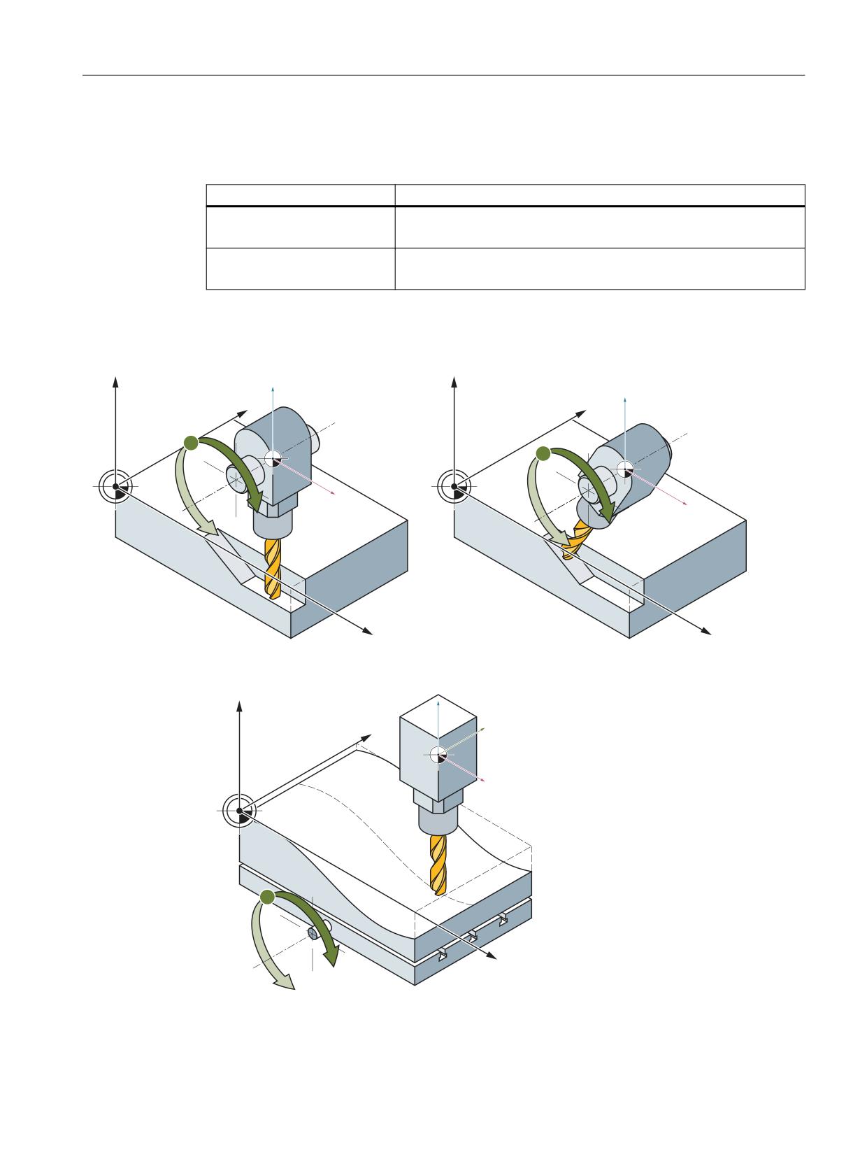
The 3 and 4-axis transformations are distinguished by the following characteristics:
Transformation
Characteristics
3-axis transformation
2 linear axes
1 rotary axis
4-axis transformation
3 linear axes
1 rotary axis
Both types of transformation belong to the orientation transformations. The orientation of the
tool must be programmed explicitly. The orientation of the tool is executed in a plane
perpendicular to the rotary axis.
=
=
=
=
<
<
%
%
;
;
;
;
Figure 6-10
Schematic diagram of a 3-axis transformation
=
=
<
<
;
%
;
Figure 6-11
Schematic diagram of a 4-axis transformation with moveable workpiece
Transformations
Function Manual, 10/2020, 6FC5397-5GP40-0BA1
253
Orientation transformations
6.5 Parameterization with machine data (conventional)
Tool orientation in zero position
Tool orientation at the zero position is the position of the tool for active machining plane
G17 AND position of the rotary axis 0 degrees
Axis assignments
The three linear axes included in the transformation are assigned to any channel axes via
machine data $MC_TRAFO_GEOAX_ASSIGN_TAB_n[0..2] and $MC_TRAFO_AXES_IN_n[0..2].
The following must apply for the assignment of channel axes to geometry axes for the
transformation:
$MC_TRAFO_GEOAX_ASSIGN_TAB_n[ 0 ] = $MC_TRAFO_AXES_IN_n[ 0 ]
$MC_TRAFO_GEOAX_ASSIGN_TAB_n[ 1 ] = $MC_TRAFO_AXES_IN_n[ 1 ]
$MC_TRAFO_GEOAX_ASSIGN_TAB_n[ 2 ] = $MC_TRAFO_AXES_IN_n[ 2 ]
The axes with corresponding index must be assigned to each other.
Parameter assignment procedure
• Enter the type of transformation according to the previous table as machine data:
$MC_TRAFO_TYPE_n
• Assign channel axes to the geometry axes of the transformation.
• For a 3-axis transformation, set the values for the axis, which is not required:
- $MC_TRAFO_GEOAX_ASSIGN_TAB_n[<geometry axis>] = 0
- $MC_TRAFO_AXES_IN_n[<geometry axis>] = 0
$MC_TRAFO_AXES_IN_n[ 4 ] = 0; → there is no 2nd rotary axis
• For a 4-axis transformation, set the following for the 3 linear axes
- $MC_TRAFO_GEOAX_ASSIGN_TAB_n[<geometry axis>] = ...
- $MC_TRAFO_AXES_IN_n[<geometry axis>] = ...
$MC_TRAFO_AXES_IN_n[ 4 ] = 0; → there is no 2nd rotary axis
Complete examples can be found in the "Example for 3 and 4-axis transformation" section.
6.5.1.5
Transformation with swiveled linear axis
General information
The orientation transformation with swiveling linear axis is similar to the 5-axis transformation
of Machine Type 3, though the 3rd linear axis is not always perpendicular to the plane defined
by the other two linear axes.
The transformation forms a separate transformation group. It can be used if one of the following
kinematics is present:
• Three Cartesian linear axes (X, Y, Z) and two orthogonal rotary axes (A, B).
• The rotary axes are parallel to two of the three linear axes.
Transformations
254
Function Manual, 10/2020, 6FC5397-5GP40-0BA1
Orientation transformations
6.5 Parameterization with machine data (conventional)
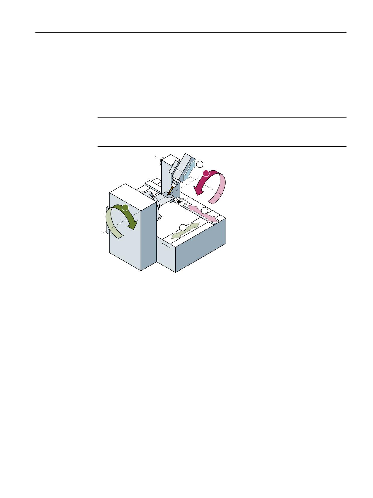
• The first rotary axis (A) is moved by two Cartesian linear axes. It rotates the third linear axis
(Z) that moves the tool.
• The tool is aligned parallel to the third linear axis (Z).
• The second rotary axis (B) rotates the workpiece.
Additional requirement:
• The first rotary axis (A) may only sweep a very small swivel range (swivel range << ± 90°).
Note
All the axis values used in the text relate to the designations of the example machine in the
following figure "Machine with swiveling linear axis Z"
$
%
① Linear axis 1 (X)
② Linear axis 2 (Y)
③ Swiveling linear axis 3 (Z)
Figure 6-12
Example: Machine with swiveling linear axis Z
Pole
The transformation with swiveling linear axis has a pole for a tool orientation parallel to the
second rotary axis (B). Singularity occurs in the pole position because the third linear axis (Z) is
parallel to the plane of the first two linear axes (X, Y), thus excluding the possibility of
compensating movements perpendicular to this plane.
Parameterizations
Kinematic variants
The kinematic variant of the machine is set in the machine data:
Transformations
Function Manual, 10/2020, 6FC5397-5GP40-0BA1
255

Orientation transformations
6.5 Parameterization with machine data (conventional)
MD24100, ... MD25190 $MC_TRAFO_TYP_n = <type>, with n = 1, 2, 3, ...
Kinematics
<type>
1st rotary axis
2nd rotary axis
swiveled linear axis
Bits 6 - 0
A
B
Z
10 00 000
A
C
Y
10 00 001
B
A
Z
10 00 010
B
C
X
10 00 011
C
A
Y
10 00 100
C
B
X
10 00 101
Machine kinematics
The machine kinematics is set for the 1st ($MC_TRAFO5 ... _1) and/or 2nd ($MC_TRAFO5 ... _2)
5-axis transformation in the channel set with the following machine data:
• Vector (po, see following figure) from the second rotary axis to workpiece table zero:
- MD24500 $MC_TRAFO5_PART_OFFSET_1
- MD24600 $MC_TRAFO5_PART_OFFSET_2
• Axis positions of the two rotary axes at the initial position of the machine:
- MD24510 $MC_TRAFO5_ROT_AX_OFFSET_1
- MD24610 $MC_TRAFO5_ROT_AX_OFFSET_2
• Sign with which the rotary axis positions are included in the transformation:
- MD24520 $MC_TRAFO5_ROT_SIGN_IS_PLUS_1
- MD24620 $MC_TRAFO5_ROT_SIGN_IS_PLUS_2
• Vector (jo) from machine zero to the second rotary axis:
- MD24560 $MC_TRAFO5_JOINT_OFFSET_1
- MD24660 $MC_TRAFO5_JOINT_OFFSET_2
• Vector (to) from the toolholder (flange) to the first rotary axis (measured at machine initial
position):
- MD24550 $MC_TRAFO5_BASE_TOOL_1
- MD24650 $MC_TRAFO5_BASE_TOOL_2
• Vector (ro) from machine zero to the first rotary axis (measured at the machine initial
position):
- MD24562 $MC_TRAFO5_TOOL_ROT_AX_OFFSET_1
- MD24662 $MC_TRAFO5_TOOL_ROT_AX_OFFSET_2
Transformations
256
Function Manual, 10/2020, 6FC5397-5GP40-0BA1
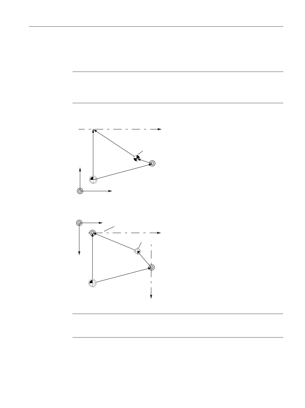
Orientation transformations
6.5 Parameterization with machine data (conventional)
Determining the machine data values
As an aid for determining the values for the above-mentioned machine data, the following two
sketches clarify the relationships between the vectors.
Note
Requirement
The machine has been traversed so that the tool holding flange aligns with the table zero (*). Is
this is technically not possible, vector to must be corrected by the deviations.
9LHZ DJDLQVW WKH ; D[LV
$[LV RI URWDWLRQ ZKLFK VZLYHOV
WKH UG OLQHDU D[LV =
UR
WR
=HUR SRLQW RI WKH WDEOH
SR
$[LV RI URWDWLRQ RI WKH
=
WDEOH
MR
0DFKLQH ]HUR SRLQW
;
<
9LHZ DJDLQVW WKH = D[LV
=
<
$[LV RI URWDWLRQ ZKLFK VZLYHOV WKH UG OLQHDU D[LV =
=
WR
:RUNSLHFH ]HUR SRLQW RQ
UR
WKH WDEOH
;
SR
MR
0DFKLQH ]HUR SRLQW
$[LV RI URWDWLRQ RI WKH
WDEOH
Figure 6-13
Projections of the vectors to be set in the machine data
Note
A physically identical point on the 1st rotary axis (e.g. point of intersection between the tool axis
and the 1st rotary axis) must be assumed for both views.
Transformations
Function Manual, 10/2020, 6FC5397-5GP40-0BA1
257
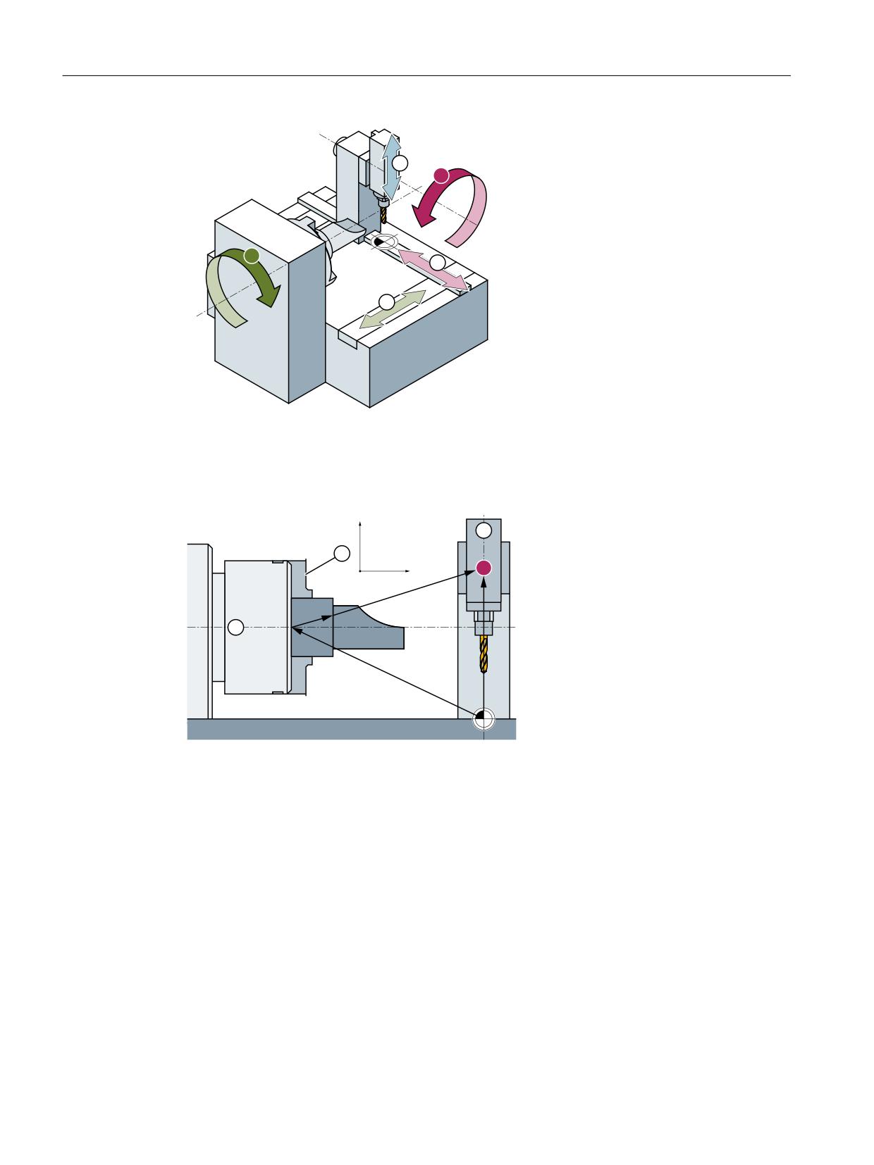
Orientation transformations
6.5 Parameterization with machine data (conventional)
$
%
① Linear axis 1 (X)
② Linear axis 2 (Y)
③ Swiveling linear axis 3 (Z)
Figure 6-14
Machine in the zero position
=
;
<
WR
SR
MR
UR]
UR
① Stand
② Fixture
③ Axis of the tool
Figure 6-15
Front view: Vectors for machine in the zero position
Transformations
258
Function Manual, 10/2020, 6FC5397-5GP40-0BA1
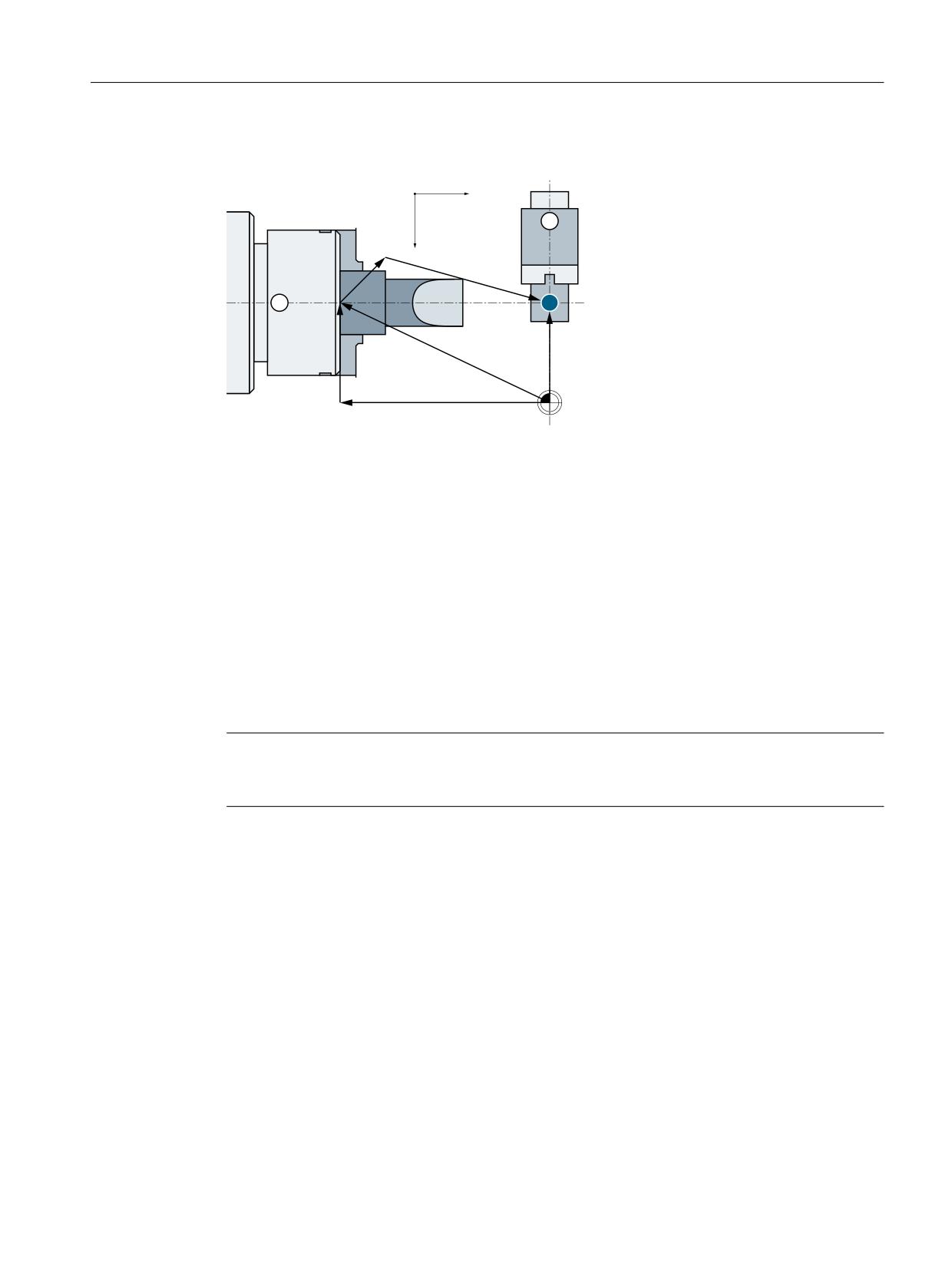
Orientation transformations
6.5 Parameterization with machine data (conventional)
<
;
WR
SR
=
MR
UR
MR
[
MR\
① Stator with clamping device
② Swivel axis of the linear axis
Figure 6-16
Top view: Vectors for machine in the zero position
Determination of the machine data values
Perform the following operation:
1. Determine, as shown in the lower part for vector jo in the "Vectors for machine in zero
position" figure, the X and Y components for all vectors.
2. As shown in the upper part for vector ro in the "Vectors for machine in zero position" figure,
determine the Z component for all vectors.
3. Enter the X, Y and Z components of the vectors (po, jo, to, ro) in the relevant machine data.
The procedure can be used all settable kinematic variants.
Note
For the appropriate machine geometry or position of the machine zero, both individual
components as well as complete vectors can become zero.
Programming
The switch on/off of the transformation in the part program or synchronized action is described
in Section "Programming of the 3- to 5-axis transformation (Page 351)".
Tool orientation
For a transformation with swiveling linear axis, the same statements as for the 5-axis
transformation with regard to the tool orientation apply similarly (see Section "Programming the
tool orientation (Page 264)").
Transformations
Function Manual, 10/2020, 6FC5397-5GP40-0BA1
259
Orientation transformations
6.6 Restrictions for kinematics and interpolation
6.6
Restrictions for kinematics and interpolation
6.6.1
Restrictions for kinematics and interpolation
For systems where there are less than six axes available for transformation, the following
restrictions must be taken into account.
5-axis kinematics
For 5-axis kinematics there are two degrees of freedom for orientation. The assignment of
orientation axes and tool vector direction must be selected so that there is no rotation around
the tool vector. As a result, only two orientation angles are required to describe the orientation.
If the axis is traversed using ORIVECT, the tool vector performs pure swiveling motion.
3-and 4-axis kinematics
For 3- and 4-axis kinematics, only one degree of freedom is available for orientation. The
respective transformation determines the relevant orientation angle. In this case, it only makes
sense to traverse the orientation axis using ORIAXES. In this case, the orientation axis is directly
and linearly interpolated.
Interpolation of the tool orientation over several blocks by means of orientation vectors
If the orientation of a tool is programmed over several consecutive part program blocks by
directly entering the appropriate rotary axis positions, then undesirable discontinuous changes
of the orientation vector are obtained at the block transitions. This results in discontinuous
velocity and acceleration changes of the rotary axes. This means that no continuous velocity and
acceleration of the orientation axes over several blocks can be achieved using large circle
interpolation.
Continuous block transitions
As long as only linear blocks (G1) are programmed, then the orientation axes also behave just
like linear axes. In this case, motion with continuous acceleration is achieved through
polynomial interpolation. Significantly better results can be achieved by programming the
orientation in space using orientation vectors (see Section "Polynomial interpolation of
orientation vectors (Page 303)").
6.6.2
Singularities of orientation
Description of problem
As described in Section "Singularities and how to treat them", singularities (poles) are
constellations in which the tool is orientated becomes parallel to the first rotary axis. If the
orientation is changed when the tool is in or close to a singularity (as is the case with large-circle
interpolation ORIWKS), the rotary axis positions must change by large amounts to achieve small
changes in orientation. In extreme cases, a jump in the rotary axis position would be needed.
Transformations
260
Function Manual, 10/2020, 6FC5397-5GP40-0BA1
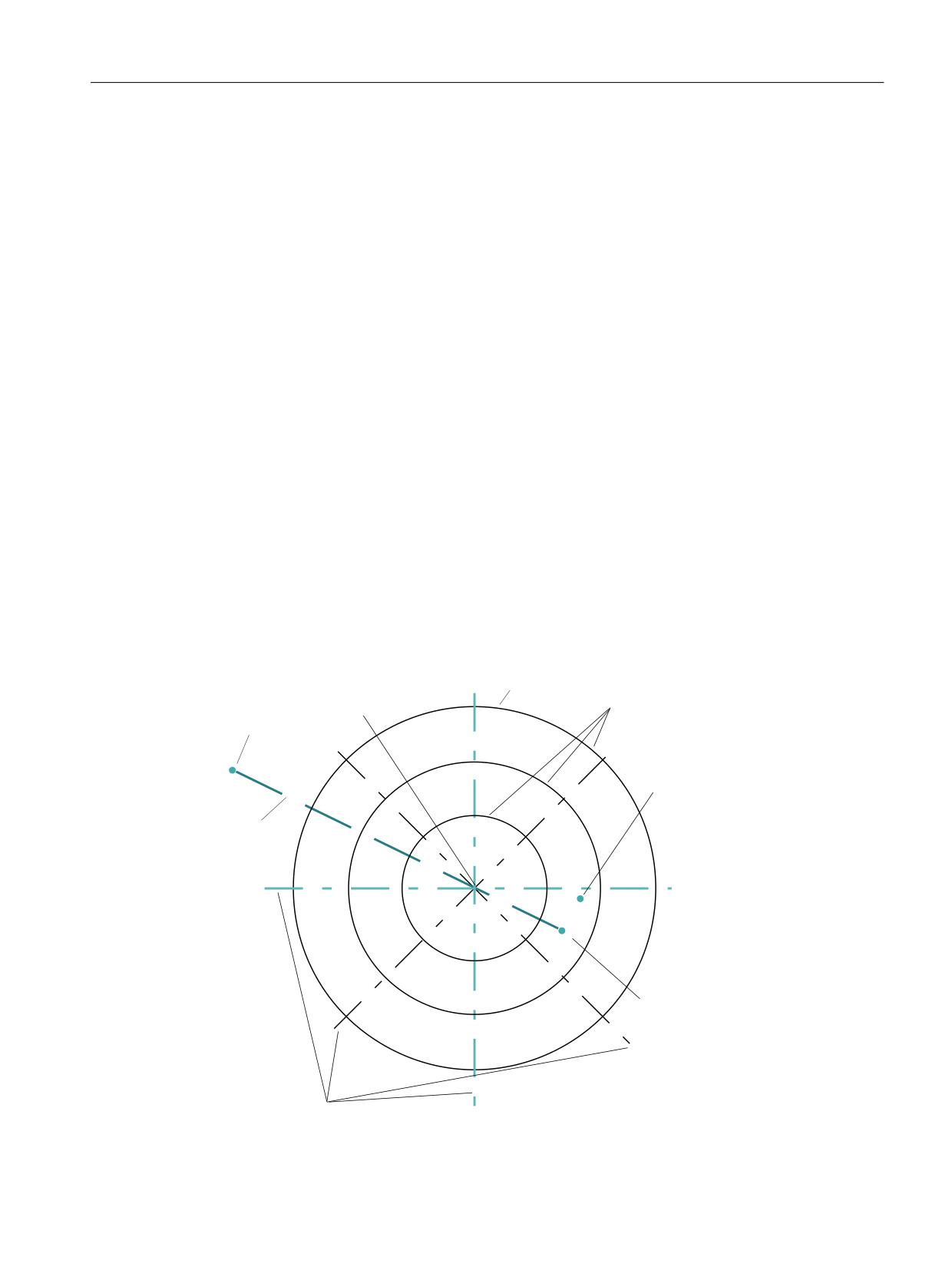
Orientation transformations
6.6 Restrictions for kinematics and interpolation
Kinematic chain:
The following system variables are relevant for kinematic chains:
• $NT_POLE_LIMIT[n] (end angle tolerance with interpolation through pole)
• $NT_POLE_TOL[n] (end angle tolerance for pole interpolation)
Conventional transformation:
The relevant machine data describes a circle around the pole:
• MD24540 $MC_TRAFO5_POLE_LIMIT_1 (closing angle tolerance for interpolation by pole for
5-axis transformation)
or
• MD24640 $MC_TRAFO5_POLE_LIMIT_2 (closing angle tolerance for interpolation by pole for
5-xis transformation)
More information
"NC Programming" Programming Manual
Example for machine type 1
Rotatable tool
Both rotary axes change the orientation of the workpiece. The orientation of the workpiece is
fixed.
2-axis swivel head with rotary axis RA 1 (4th transformation axis) and rotary axis RA 2 (5th
transformation axis).
7ROHUDQFH FLUFOH
&RQVWDQW
3ROH
3RVLWLRQ RI WKH
QG URWDU\ D[LV
6WDUW SRLQW
3URJUDP
PHG
(QG SRLQW
3DWK
UHDFKHG
(QG SRLQW
&RQVWDQW
3RVLWLRQ RI WKH
VW URWDU\ D[LV
Transformations
Function Manual, 10/2020, 6FC5397-5GP40-0BA1
261
Orientation transformations
6.7 Orientation
Figure 6-17
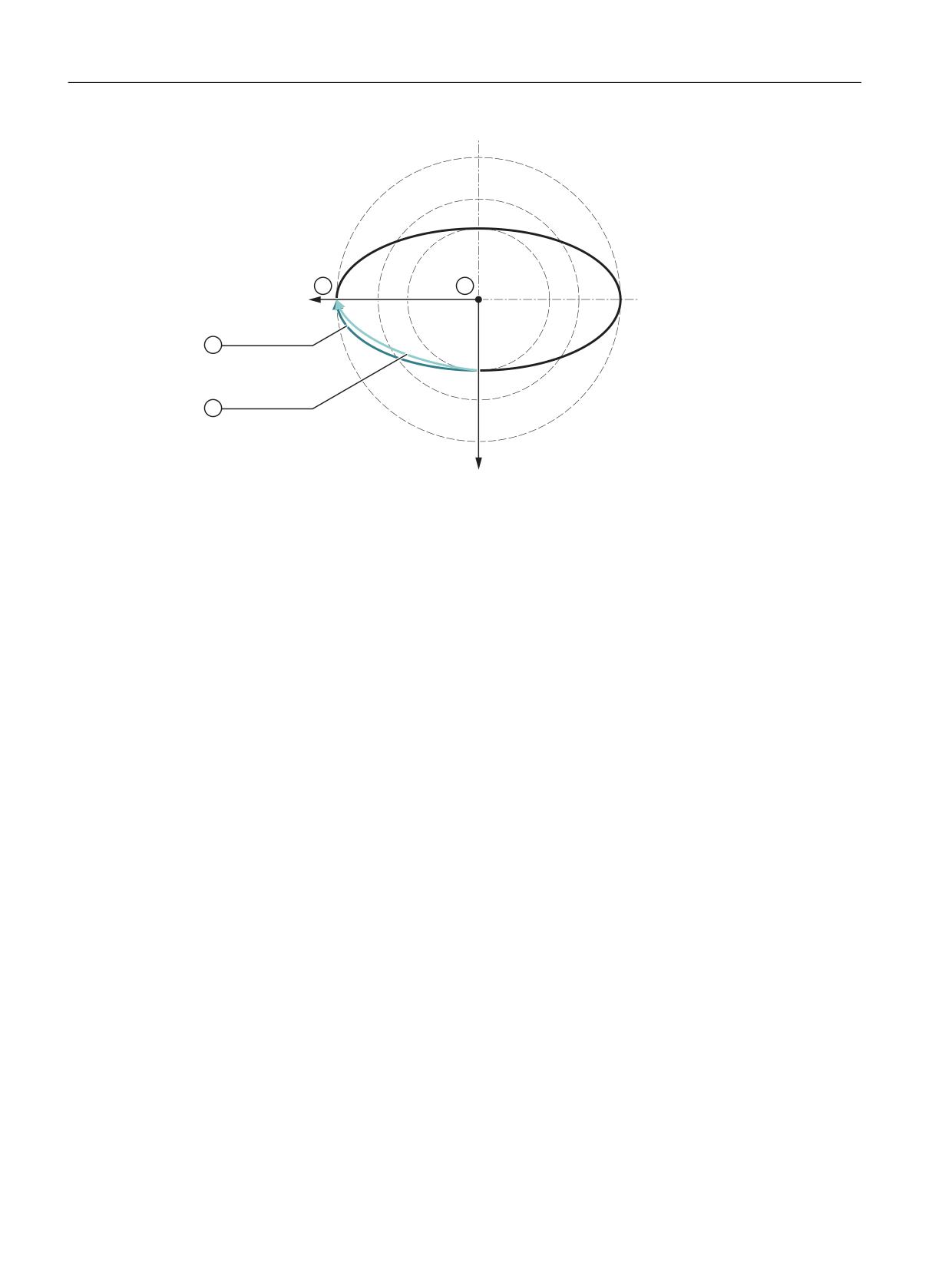
Generic 5-axis transformation; end point of orientation inside tolerance circle.
End point within the circle
If the end point is within the circle, the first axis comes to a standstill and the second axis moves
until the difference between target and actual orientation is minimal. However, since the first
rotary axis does not move, the orientation will generally deviate from the programmed value
(see previous figure). However, the programmed orientation can at least be reached exactly if
the first rotary axis happens to be positioned correctly.
Note
In the previous figure, the resulting path is a straight line because the position of the first rotary
axis is constant on that path. This representation is always correct, irrespective of the angle
between the two rotary axes. The orientation vector only moves in a plane, however, if the two
rotary axes and the basic orientation are all mutually perpendicular. In all other cases, the
orientation vector describes the outside of a cone.
End point outside the circle
If the orientation interpolation describes a path through the circle, while the end point is outside
the circle, the end point is approached with axis interpolation. This applies in particular if the
interpolation starting point is located inside the circle. Path deviations from the programmed
setpoint orientation are thus unavoidable.
6.7
Orientation
6.7.1
Definition of orientation vectors
Tool orientation
For the purpose of 5-axis machining, the orientation of the tool needs to be defined in addition
to the position setpoint of the machining point. There are a variety of methods that are
commonly used to define the tool orientation.
Transformations
262
Function Manual, 10/2020, 6FC5397-5GP40-0BA1
Orientation transformations
6.7 Orientation
Description of tool orientation
The tool orientations can be programmed in the following ways:
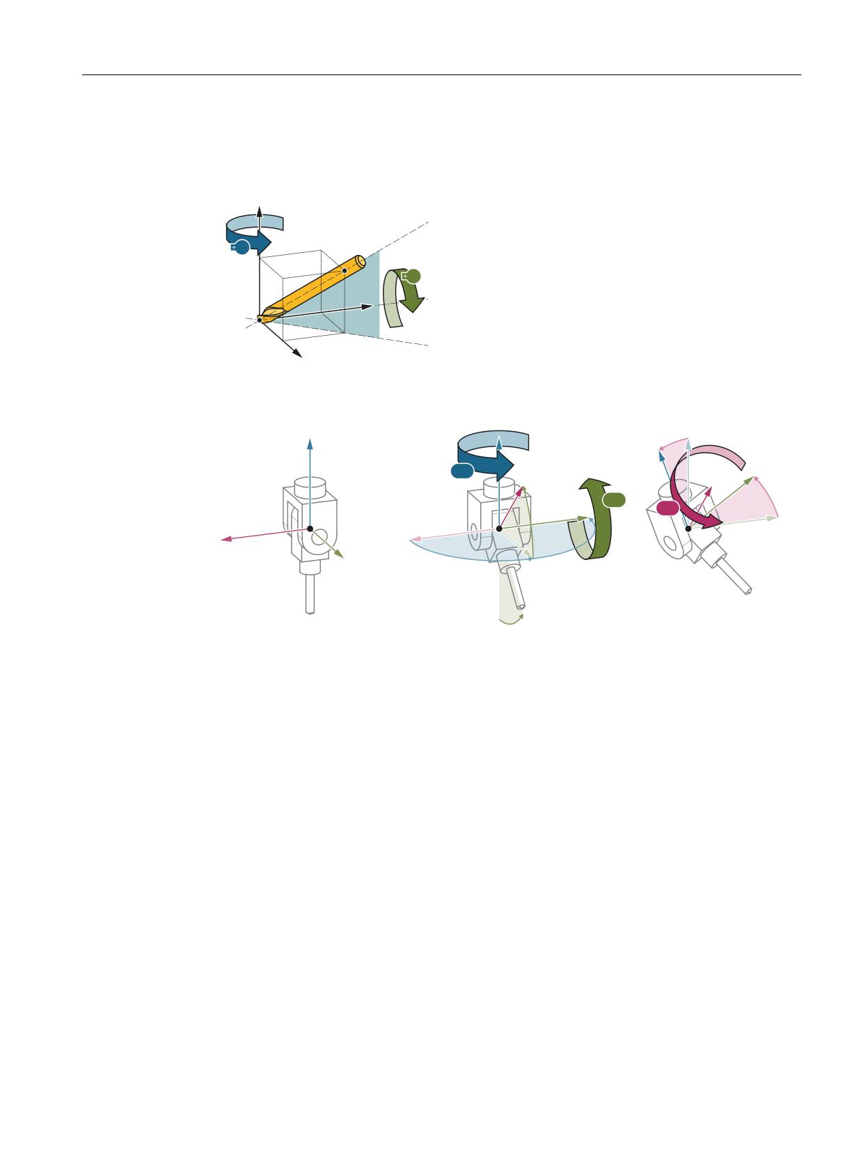
1. Programming of rotary axis positions with A, B and C or with the actual rotary axis names.
;
$
#
:
9
Figure 6-18
Rotary axis position
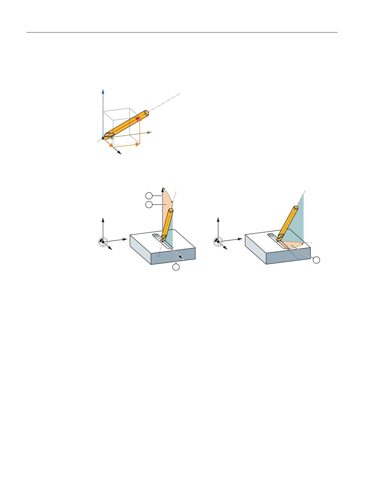
2. Programming in Euler angle or RPY angle via A2, B2, C2
;
;
;
$
9݁
9݁
#
:݀
"
:݀
9
:
Figure 6-19
Euler RPY angle
Transformations
Function Manual, 10/2020, 6FC5397-5GP40-0BA1
263
Orientation transformations
6.7 Orientation
3. Programming of the direction vector via A3, B3, C3.
An orientation vector can be programmed in each block. If polynomials are programmed for
the orientation, the interpolated orientation vector is generally turned not in the plane
between start and end vector, but it can be rotated at random from this plane.
;
$
:
"
#
9
Figure 6-20
Orientation vector
4. Programming using lead angle LEAD and tilt angle TILT.
;
;
:
:
9
9
① Surface normal vector B
② Path tangent A
③ Lead angle LEAD
④ Tilt angle TILT at end of block
Figure 6-21
Lead/tilt
6.7.2
Programming the tool orientation
For multi-axis machining with tools at an angle or for milling any geometries positioned in space,
3 linear axes X, Y and Z and a combination of two additional rotary axes A, B, C are required. It
must be possible to control the axes simultaneously. Using three linear axes and two rotary axes,
theoretically any point in space can be approached with any tool orientation.
For orientation interpolations, the orientation of the tool needs to be defined in addition to the
position setpoint of the machining point.
Transformations
264
Function Manual, 10/2020, 6FC5397-5GP40-0BA1
Orientation transformations
6.7 Orientation
=
$
;
%
<
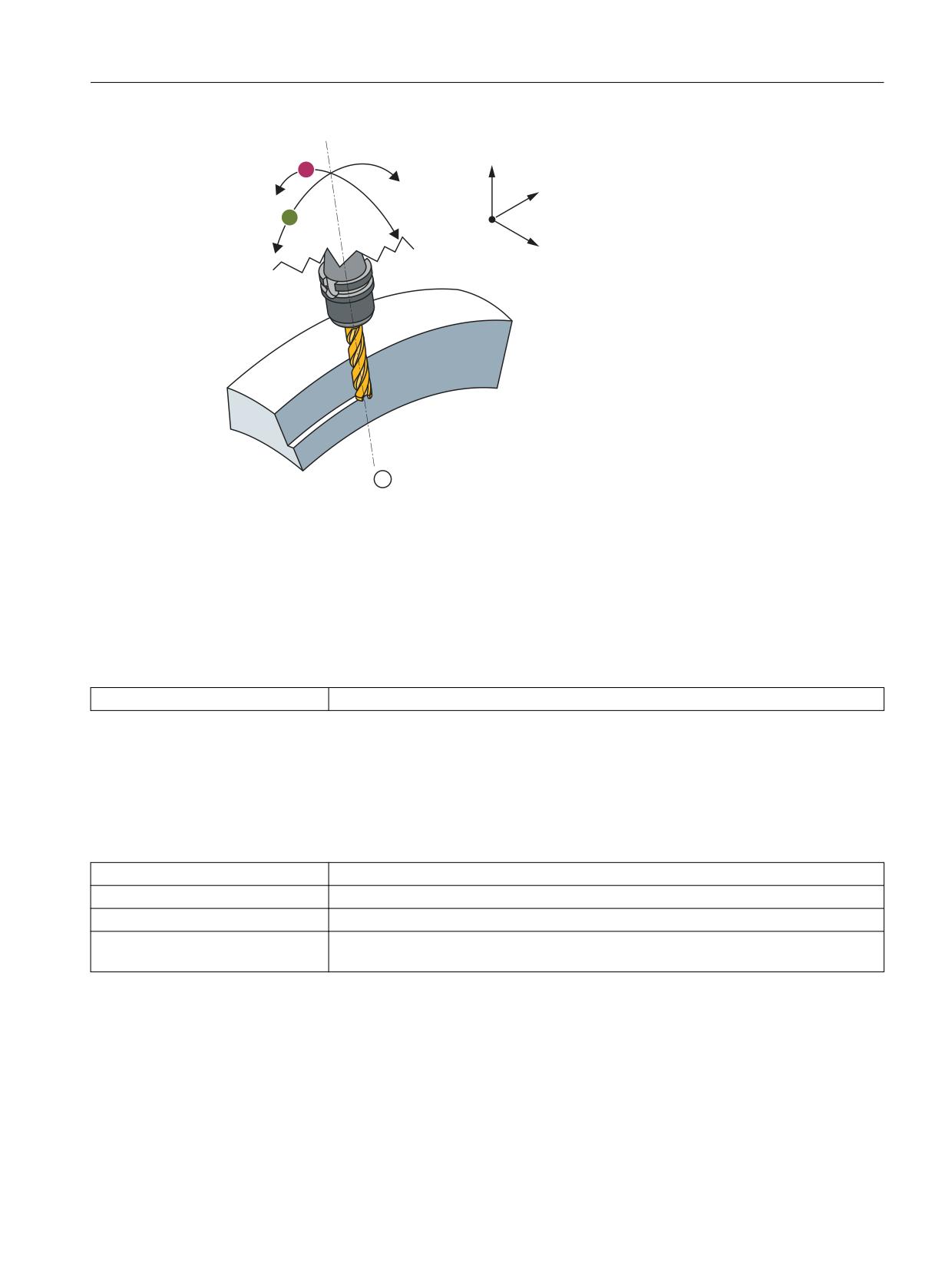
① Tool axis
Figure 6-22
Processing of workpieces with 5-axis transformation
Programming of tool orientations for machine-related orientation
The tool orientation is described in relation to the machine coordinate system (MCS). The tool
is programmed in its alignment to the machine and is therefore
dependent on the machine kinematics. Programming is done by specifying:
A, B, C
Direct specification of rotary axis positions
Programming of tool orientations for workpiece-related orientation
The orientation of the tool can be programmed in a block directly by specifying the rotary axes
or indirectly by specifying the Euler angle, RPY angle and direction vector.
The following options are available:
A2, B2, C2
Angle programming of virtual axes via Euler angles or RPY angles
A3, B3, C3
Vector component designation
LEAD, TILT
Specification of lead and tilt angles with reference to path and surface
A4, B4, C4
Surface normal vectors at the start of the block and at the end of the block
A5, B5, C5
The identifiers for Euler angles and direction vectors can be set in machine data:
Euler angles via:
MD10620 $MN_EULER_ANGLE_NAME_TAB (name of Euler angles)
Direction vector via:
MD10640 $MN_DIR_VECTOR_NAME_TAB (name of direction vectors)
Transformations
Function Manual, 10/2020, 6FC5397-5GP40-0BA1
265
Orientation transformations
6.7 Orientation
The tool orientation can be located in any block. Above all, it can be programmed alone in a
block, resulting in a change of orientation in relation to the tool tip which is fixed in its
relationship to the workpiece.
Euler or RPY
The following machine data can be used to switch between Euler and RPY angles:
MD21100 $MC_ORIENTATION_IS_EULER (angle definition for orientation programming)
Orientation reference
A tool orientation at the start of a block can be transferred to the block end in two different ways:
• in the workpiece coordinate system with command ORIWKS
• in the machine coordinate system with command ORIMKS
ORIWKS command
The tool orientation is programmed in the workpiece coordinate system (WCS) and is thus not
dependent on the machine kinematics.
In the case of a change in orientation with the tool tip at a fixed point in space, the tool moves
along a large arc on the plane stretching from the start vector to the end vector.
ORIMKS command
The tool orientation is programmed in the machine coordinate system and is thus dependent on
the machine kinematics.
In the case of a change in orientation of a tool tip at a fixed point in space, linear interpolation
takes place between the rotary axis positions.
The orientation is selected via NC language commands ORIWKS and ORIMKS.
Transformations
266
Function Manual, 10/2020, 6FC5397-5GP40-0BA1
Orientation transformations
6.7 Orientation
=
r
)
$
;
%
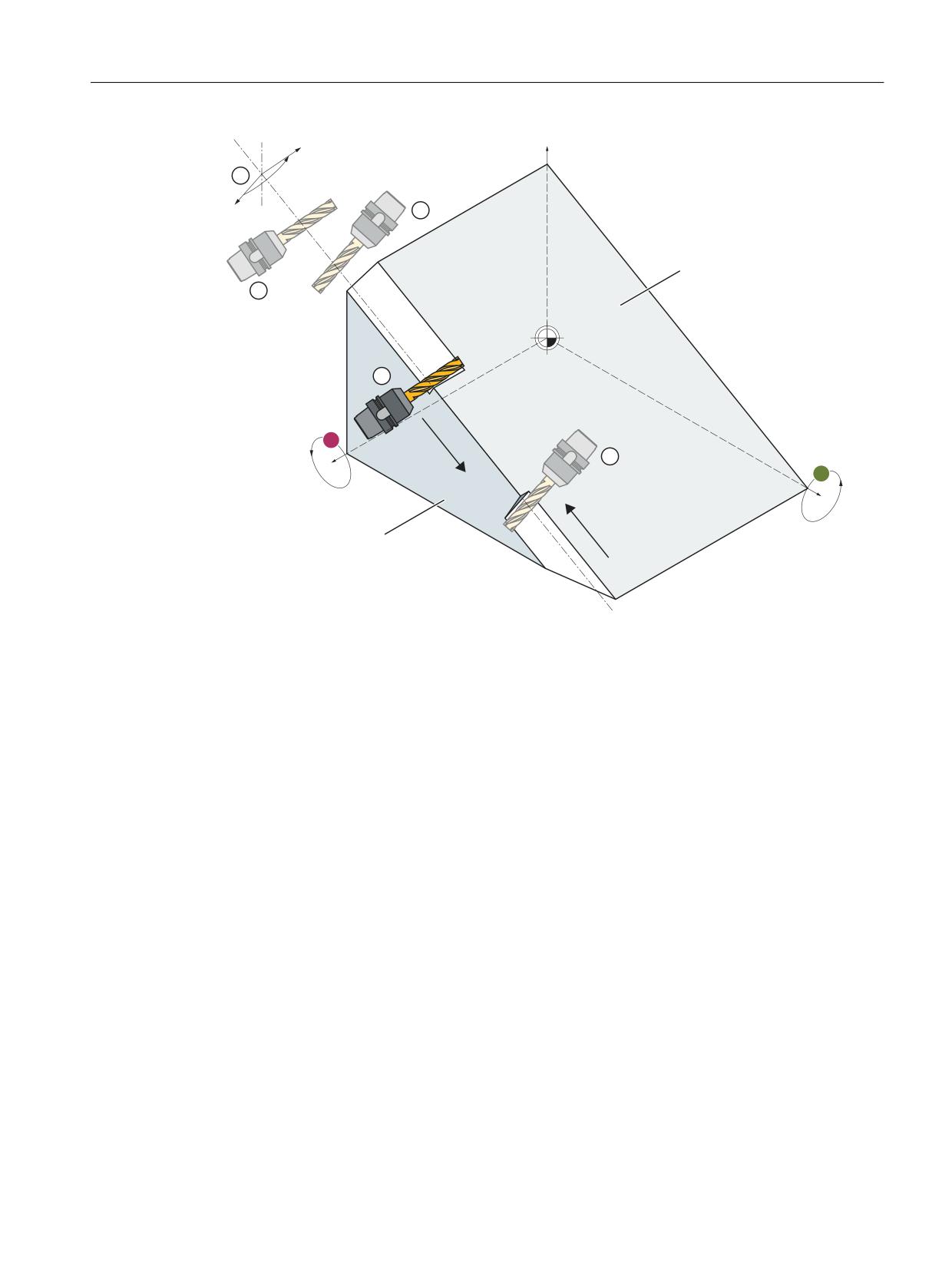
<
)
① Process the surface F1 along the edge of F2
② Retraction
③ Orientation change B: +90° A: -30°
④ Approach of area F2
⑤ Process the surface F2 along the edge of F1
Figure 6-23
Change in cutter orientation while processing inclined edges
Transformations
Function Manual, 10/2020, 6FC5397-5GP40-0BA1
267
Orientation transformations
6.7 Orientation
r
r
r
;
=
<
② Retraction
③ with ORIWKS (large circle)
④ Approach of area F2
⑤ With ORIMKS (linear interpolation between rotary axes)
Figure 6-24
Change in orientation while processing inclined edges
ORIMKS constitutes the basic setting
The basic setting can be changed via the following machine data:
MD20150 MC_GCODE_RESET_VALUES (RESET position of G groups)
MD20150 $MC_GCODE_RESET_VALUES [24] = 1 ⇒ ORIWKS is basic setting
MD20150 $MC_GCODE_RESET_VALUES [24] = 2 ⇒ ORIWKS is basic setting
Illegal tool orientation
If tool position is programmed in relation to the following functions, alarm 12130 "Illegal tool
orientation" is output when Euler angles and direction vectors are selected and the NC program
then stops (this alarm can also occur in connection with G331, G332 and G63).
• G04: Dwell time
• G33: Thread cutting with constant lead
• G74: Approaching a reference point
• G75: Approaching a fixed point
• REPOSL: Repositioning to the contour
• REPOSQ: Repositioning to the contour
• REPOSH: Repositioning to the contour
To remedy this situation, tool orientation can be programmed with axis end values.
Transformations
268
Function Manual, 10/2020, 6FC5397-5GP40-0BA1
Orientation transformations
6.7 Orientation
Alarm 17630 or 17620 is output for G74 and G75 if a transformation is active and the axes to be
traversed are involved in the transformation. This applies irrespective of orientation
programming.
If the start and end vectors are inverse parallel when ORIWKS is active, then no unique plane is
defined for the orientation programming, resulting in the output of alarm 14120.
If a transformation switch (switch On, switch Off or change transformation) is undertaken,
alarm 14400 will be generated.
In the reverse situation, i.e. a tool radius offset is selected or deselected when a transformation
is active, no alarm message is output.
Multiple input of tool orientation
According to DIN 66025, only one tool orientation may be programmed in a block, e.g. with
direction vectors:
N50
A3=1 B3=1 C3=1
If tool orientation is entered multiply, i.e. with direction vectors and with Euler angles, error
message 12240 "Channel X block Y tool orientation xx defined more than once" is displayed and
the NC part program stops.
N60
A3=1 B3=1 C3=1
A2=0 B2=1 C2=3
Tool orientation using orientation vectors
Polynomials can also be programmed for the modification of the orientation vector.
This method produces an extremely smooth change in speed and acceleration at the block
changes for rotary axes when the tool orientation has to be programmed over several blocks.
The interpolation of orientation vectors can be programmed with polynomials up to the 5th
degree. Polynomial interpolation of orientation vectors is described in Chapter "Polynomial
interpolation of orientation vectors (Page 303)".
Note
Further explanations of tool orientation using orientation vectors and their handling in
machines are given in:
More information
Function Manual Tools, tool offset, orientable tool carriers
Transformations
Function Manual, 10/2020, 6FC5397-5GP40-0BA1
269
Orientation transformations
6.7 Orientation
6.7.3
Basic orientation with kinematic chain
Basic orientation for orientation transformations
For orientation transformations, the basic tool orientation is specified via the system variables
$NT_BASE_ORIENT or $NT_BASE_ORIENT_NORMAL. The orientations come into effect if no tool
is selected. If the vectors are not explicitly defined, the default setting is (0, 0, 1).
• $NT_BASE_ORIENT[n, 0 ...2]; defines the basic tool orientation via a vector, as shown in the
following example:
- $NT_BASE_ORIENT[1, 0] = 1.0; component in X-direction
- $NT_BASE_ORIENT[1, 1] = 1.5; component in Y-direction
- $NT_BASE_ORIENT[1, 2] = 100; component in Z-direction
• $NT_BASE_ORIENT_NORMAL[n, 0 ...2] defines a vector which stands vertically on the basic
tool orientation for orientation transformations with three degrees of freedom. If the vectors
are not explicitly defined, the default setting is (0, 1, 0).
• $NT_IGNORE_TOOL_ORIENT[n]; if the system variable is set, the values from the system
variables $NT_BASE_ORIENT and $NT_BASE_ORIENT_NORMAL are also used when a tool is
active.
If an orientation is programmed by means of Euler angles, RPY angles (A2, B2, C2) or vectors (A3,
B3, C3), basic orientation is taken into consideration, i.e. the rotary axes are positioned so that
a tool positioned in basic orientation is traversed to the programmed orientation.
If the rotary axes are programmed directly, basic orientation has no effect on this.
Active tool
If a tool is active, the basic orientation is determined by the orientation valid for the tool. This can
be defined as required and deviating from the standard (orientation in the direction of the
coordinate axes depending on the active G code of group 6, G17 - G19) with the aid of the tool
parameters $TC_DPV. This option is particularly important when using angled tools, where, for
example, the tool points in the X direction although G17 is active.
More information:
Function Manual, Tool Management
The scope of functions does not differ from the scope of functions of conventional orientation
transformations (TRAORI).
6.7.4
Basic orientation for conventional transformations
Basic orientation for 5-axis transformations
For 5-axis transformations, the basic orientation of the tool is determined by the transformation
type.
Transformations
270
Function Manual, 10/2020, 6FC5397-5GP40-0BA1
Orientation transformations
6.7 Orientation
Generic 5-axis transformation can be used to enable any basic tool orientation, i.e. space
orientation of the tool is arbitrary, with axes in their initial positions.
If an orientation is programmed by means of Euler angles, RPY angles (A2, B2, C2) or vectors (A3,
B3, C3), basic orientation is taken into consideration, i.e. the rotary axes are positioned so that
a tool positioned in basic orientation is traversed to the programmed orientation.
If the rotary axes are programmed directly, basic orientation has no effect on this.
Definition
The basic orientation can be defined in three different ways:
• Definition by calling the transformation
• Definition by the orientation of the active tool
• Definition using a machine data
Definition by calling the transformation
When the transformation is called, the direction vector of the basic orientation can be specified
in the call, e.g. TRAORI(0, 0., 1., 5.). The direction vector is defined by parameters 2 to
4. This is the reason that in the example it has the value (0., 1., 5.).
The first parameter specifies the transformation number. The number can be omitted if the first
transformation is to be activated. To enable the parameters to be identified correctly when
specifying an orientation, a blank space has to be inserted instead of the transformation
number, e.g. TRAORI(, 0., 1., 5.).
Note
The orientation data is absolute. It is not modified by a frame that is possibly active.
The absolute value of the vector is insignificant, only the direction is relevant. Non-programmed
vector elements can be set to zero.
Please note that if all three vector components are zero (because they have been set explicitly
so or not specified at all), the basic orientation is not defined by data in the TRAORI(...) call,
but by one of the two other options.
If a basic orientation is defined by calling the transformation, it cannot be altered while a
transformation is active. The orientation can be changed only by selecting the transformation
again.
Definition by the orientation of the active tool
The basic orientation is determined by the tool, if:
• it has not been defined by specifying a direction vector in the transformation call
and
• a tool is already active.
The orientation of a tool is dependent on the selected plane. It is parallel to Z at G17, parallel to
Y at G18 and parallel to X at G19.
Transformations
Function Manual, 10/2020, 6FC5397-5GP40-0BA1
271
Orientation transformations
6.7 Orientation
It can be modified arbitrarily by orientable toolholders, see:
More information
Function Manual Tools; Tool offset, orientable tool carriers
If the tool is changed when a transformation is active, the basic orientation is also updated. The
same applies if the orientation of a tool changes as the result of a change in plane (plane changes
are equivalent to tool changes, as they also alter the assignment between tool length
components and individual axes).
If the tool is de-selected, thereby canceling the definition of tool orientation, the basic
orientation programmed in machine data becomes operative.
Definition using a machine data
If the basic orientation is not defined by either of the two variants described above, it is specified
with reference to the following machine data:
$MC_TRAFO5_BASE_ORIENT_n (basic tool orientation)
This machine data must not be set to a zero vector or else an alarm will be generated during
control run-up when a transformation is active.
If a basic orientation is programmed in machine data $MC_TRAFO5_BASE_ORIENT_n when a
transformation is active and a tool is subsequently activated, the basic orientation is re-defined
by the tool.
Note
The range of settable orientations depends on the directions of the rotary axes involved and the
basic orientation. The rotary axes must be mutually perpendicular if all possible orientations are
to be used. If this condition is not met, "dead" ranges will occur.
Examples:
1. Extreme example: A machine with rotatable tool has a C axis as its first rotary axis and an A
axis as its second. If the basic orientation is defined in parallel to the A axis, the orientation
can only be changed in the X-Y plane (when the C axis is rotating), i.e. orientation with a Z
component unequal to zero is not possible in this instance. The orientation does not change
when the A axis rotates.
2. Realistic example: A machine with nutator kinematics (cardan head) with an axis inclined at
less than 45o in a basic orientation parallel to the Z axis can only assume orientations within
a semi-circle: The top semi-circle with basic orientation towards +Z and the bottom with basic
orientation towards -Z.
6.7.5
Orientation movements with axis limits
Calculate rotary axis position
If the final orientation in a 5-axis transformation is programmed indirectly in an NC block by
means of a Euler, RPY angle or direction vector, it is necessary to calculate the rotary axis
positions that produce the desired orientation. This calculation has no unique result.
Transformations
272
Function Manual, 10/2020, 6FC5397-5GP40-0BA1

Orientation transformations
6.7 Orientation
There are always at least two essentially different solutions. In addition, any number of solutions
can result from a modification to the rotary axis positions by any multiple of 360 degrees.
The control system chooses the solution which represents the shortest distance from the current
starting point, allowing for the programmed interpolation type.
Specify axis limits (kinematic chains)
The minimum or the maximum position of a rotary axis can be defined via the system
variables $NT_ROT_AX_MIN (Page 244) and $NT_ROT_AX_MAX (Page 245).
Note
The system variables are only evaluated if both values are not equal to "0".
Determining permissible axis limits (conventional transformation)
The control system attempts to define another permissible solution if the axis limits are violated,
by approaching the desired axis position along the shortest path. The second solution is then
verified, and if this solution also violates the axis limits, the axis positions for both solutions are
modified by multiples of 360 until a valid position is found.
The following conditions must be met in order to monitor the axis limits of a rotary axis and
modify the calculated end positions:
• A generic 5-axis transformation of type 24, 40 or 56 must be active.
• The axis must be referenced.
• The axis must not be a modulo rotary axis.
• The following machine data may not be equal to zero:
MD21180 $MC_ROT_AX_SWL_CHECK_MODE (check software limits for orientation axes)
MD21180 $MC_ROT_AX_SWL_CHECK_MODE specifies the conditions under which the rotary
axis positions may be modified:
Value
Meaning
0
No modification permitted (default, equivalent to previous behavior).
1
Modification is only permitted if axis interpolation is active (ORIAXES or ORIMKS).
2
Modification is always permitted, even if vector interpolation (large circle interpolation, conical
interpolation, etc.) was active originally.
Switch-over to axis interpolation
If the axis positions have to be changed from the originally determined value, the system
switches to rotary axis interpolation because the original interpolation path, e.g. large circle
interpolation or conical interpolation, can no longer be maintained.
Transformations
Function Manual, 10/2020, 6FC5397-5GP40-0BA1
273
Orientation transformations
6.7 Orientation
Example
An example for modifying the rotary axis motion of a 5-axis machine with a rotatable tool is
shown in Chapter "Example of generic 5-axis transformation (Page 365)".
6.7.6
Orientation compression
Function
Using compressor functions COMPON, COMPCURV, COMPCAD and COMPSURF, NC programs, in
which the orientation is programmed using direction vectors, can be compressed, but still
maintaining a specifiable tolerance.
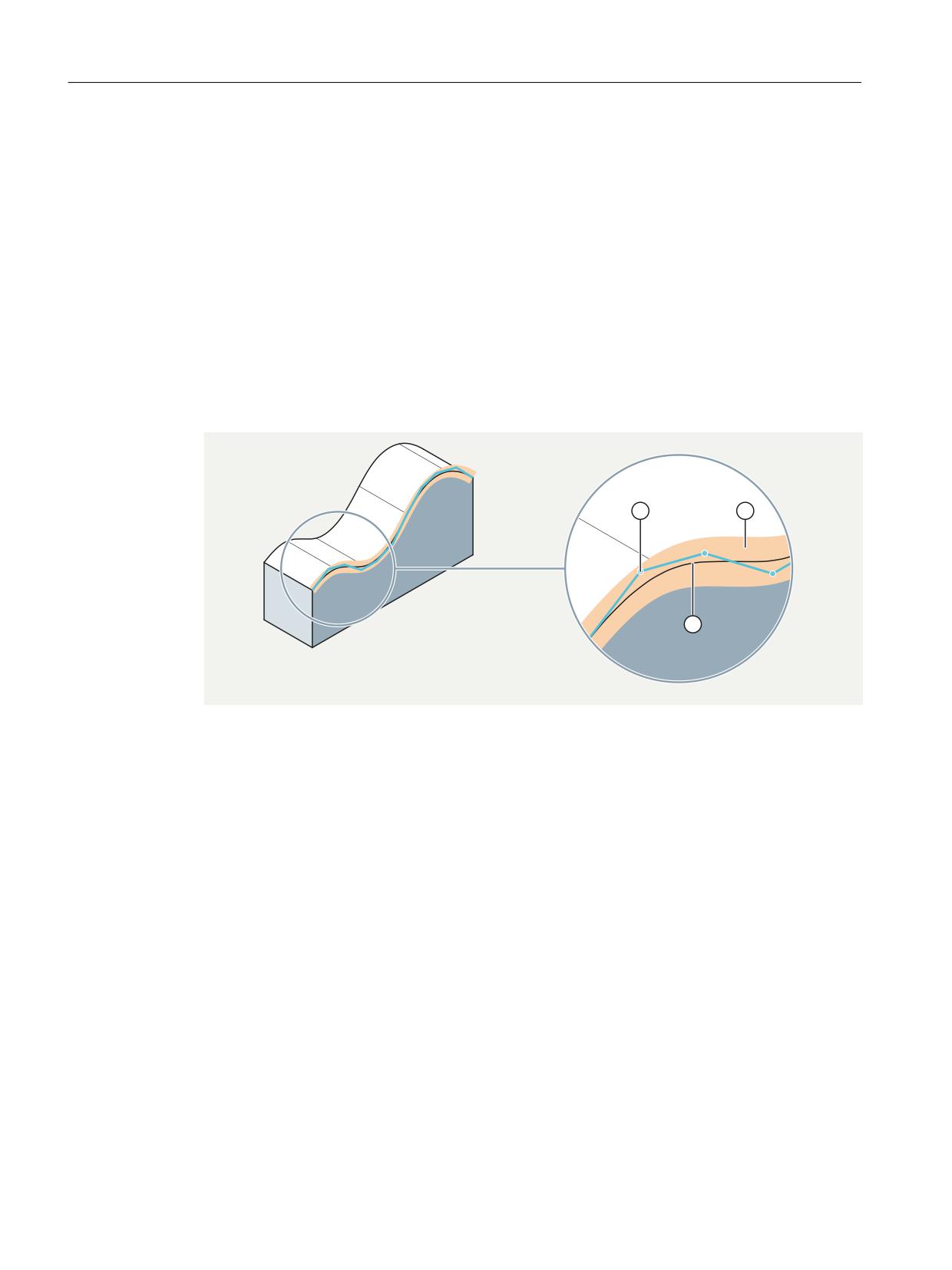
① Tolerance band
② Sequence of G1 commands
③ Resulting spline
Figure 6-25
Example compressor COMPCAD
Transformations
274
Function Manual, 10/2020, 6FC5397-5GP40-0BA1
Orientation transformations
6.7 Orientation
Requirement
An orientation motion is only compressed under the following conditions:
• Orientation transformation (TRAORI, TRAORI_DYN, TRAORI_STAT) is active.
• Large-radius circular interpolation is active.
I.e. tool orientation is changed in the plane that is determined by start and end orientation.
Large-radius circular interpolation is performed under the following conditions:
- MD21104 $MC_ORI_IPO_WITH_G_CODE = 0
+ ORIWKS is active.
+ orientation is programmed using vectors (with A3, B3, C3 or A2, B2, C2).
- MD21104 $MC_ORI_IPO_WITH_G_CODE = 1
+ ORIVECT or ORIPLANE is active.
The tool orientation can be programmed either as a direction vector or with rotary axis
positions. Large-radius circular interpolation is not executed if G command ORICONxx or
ORICURVE is active or if polynomials for orientation angle (PO[PHI] and PO[PSI]) are
programmed.
Parameterization
NC blocks can only be compressed if deviations are allowed between the programmed contour
and interpolated contour or between the programmed orientation and interpolated orientation.
Compression tolerances can be used to set the maximum permissible deviation. The higher the
tolerances, the more blocks can be compressed. However, the higher the tolerances, the more
the interpolated contour or orientation can deviate from the programmed values.
Axis accuracy
For each programmed path, the compressor generates a spline curve such that, for the axes
involved, the maximum tolerance set with the machine data is complied with in the endpoints:
MD33100 $MA_COMPRESS_POS_TOL = <maximum deviation with compression>
Contour accuracy
The maximum deviation from the programmed contour and tool orientation permitted during
compression is set with the following setting data:
• SD42475 $SC_COMPRESS_CONTUR_TOL = <maximum contour deviation>
• SD42476 $SC_COMPRESS_ORI_TOL = <maximum angular deviation of the tool orientation>
Only effective with orientation transformation.
• SD42477 $SC_COMPRESS_ORI_ROT_TOL = <maximum angular deviation of the tool
orientation>
Only effective with orientation transformation in conjunction with 6-axis transformation.
Note
A maximum deviation of tool orientation can only be specified if an orientation transformation
is active (TRAORI).
Transformations
Function Manual, 10/2020, 6FC5397-5GP40-0BA1
275

Orientation transformations
6.7 Orientation
Compression mode
With the machine data MD20482 $MC_COMPRESSOR_MODE, the following functions are
parameterized with decimal coding:
• Units digit: Taking into account tolerances
• Tens digit: Compression of blocks with programmed tool orientation and / or value
assignments.
• Hundreds digit: Compression of blocks, except linear blocks (G1).
• Thousands digit: Compression for specific applications.
MD20482 $MC_COMPRESSOR_MODE = <value>
Val-
Meaning
ue
Units digit
(Effective tolerance specifications)
xxx0
Geometry and orientation axes
MD33100 $MA_COMPRESS_POS_TOL
xxx1
Geometry axes
SD42475 $SC_COMPRESS_CONTUR_TOL
Orientation axes
MD33100 $MA_COMPRESS_POS_TOL
xxx2
Geometry axes
MD33100 $MA_COMPRESS_POS_TOL
Orientation axes
SD42476 $SC_COMPRESS_ORI_TOL
SD42477 $SC_COMPRESS_ORI_ROT_TOL
xxx3
Geometry axes
SD42475 $SC_COMPRESS_CONTUR_TOL
Orientation axes
SD42476 $SC_COMPRESS_ORI_TOL
SD42477 $SC_COMPRESS_ORI_ROT_TOL
Tens digit
(Compression of blocks with programmed tool orientation and / or value assignments)
xx0x
Blocks with programmed tool orientation and/or value assignments are compressed.
xx1x
Blocks with programmed tool orientation are compressed.
Blocks with value assignments are not compressed.
xx2x
Blocks with value assignments are compressed.
Blocks with programmed tool orientation are not compressed.
xx3x
Blocks with programmed tool orientation and / or value assignments are not compressed.
Hundreds digit
(Compression of blocks, except linear blocks (G1))
x0xx
Circular blocks and G0 blocks are not compressed.
x1xx
Circular blocks are linearized and compressed by COMPCAD.
x2xx
G0 blocks 1) are compressed.
x3xx
Circular blocks and G0 blocks 1) are compressed.
Thousands digit
(Compression for specific applications)
Transformations
276
Function Manual, 10/2020, 6FC5397-5GP40-0BA1

Orientation transformations
6.7 Orientation
0xxx
Optimization regarding the surface quality in tool and mold making.
1xxx
Optimization regarding smooth and quick traversal.
Relevant for applications such as tape laying.
1)
Another tolerance may be effective for the compression of G0 blocks as the tolerance for G0 blocks can
be preset for specific channels using machine data, and can also be adapted temporarily through
programming in the part program.
Programming
Tool orientation
If orientation transformation (TRAORI) is active, for 5-axis machines, tool orientation can be
programmed in the following way (independent of the kinematics):
• Programming of the direction vector via:
A3=<...> B3=<...> C3=<...>
• Programming of the Eulerangles or RPY-angles via:
A2=<...> B2=<...> C2=<...>
Rotation of the tool
For 6-axis machines you can program the tool rotation in addition to the tool orientation.
The angle of rotation is programmed with:
THETA=<...>
Note
NC blocks, in which rotation is also programmed, can only be compressed if the angle of rotation
changes linearly. I.e., an angle of rotation must not be programmed with a polynomial
PO[THT]=(...).
General structure of a compressible NC block
The general structure of an NC block that can be compressed can therefore look like this:
N... X=<...> Y=<...> Z=<...> A3=<...> B3=<...> C3=<...> THETA=<...> F=<...>
or
N... X=<...> Y=<...> Z=<...> A2=<...> B2=<...> C2=<...> THETA=<...> F=<...>
Programming tool orientation using rotary axis positions
Tool orientation can be also specified using rotary axis positions, e.g. with the following
structure:
N... X=<...> Y=<...> Z=<...> A=<...> B=<...> C=<...> THETA=<...> F=<...>
In this case, compression is executed in two different ways, depending on whether large-radius
circular interpolation is executed. If no large-radius circular interpolation takes place, then the
compressed change in orientation is represented in the usual way by axial polynomials for the
rotary axes.
Transformations
Function Manual, 10/2020, 6FC5397-5GP40-0BA1
277
Orientation transformations
6.7 Orientation
Activate compressor function
Compressor functions are activated by modal G commands COMPON, COMPCURV, COMPCAD or
COMPSURF.
Deactivate compressor function
COMPOF terminates the compressor function.
Example
In the example program below, a circle approximated by a polygon definition is compressed. The
tool orientation moves on the outside of the taper at the same time. Although the programmed
orientation changes are executed one after the other, but discontinuously, the compressor
function generates a smooth motion of the orientation.
Program code
Comment
DEF INT NUMBER=60
DEF REAL RADIUS=20
DEF INT COUNTER
DEF REAL ANGLE
N10 G1 X0 Y0 F5000 G64 //sort match
rate lower first
$SC_COMPRESS_CONTUR_TOL=0.05
; Maximum deviation of the contour = 0.05 mm
$SC_COMPRESS_ORI_TOL=5
; Maximum deviation of the orientation
= 5 degrees
TRAORI
COMPCURV
; The movement describes a circle generated
from polygons. The orientation moves on a
taper around the Z axis with an opening an-
gle of 45 degrees.
N100 X0 Y0 A3=0 B3=-1 C3=1
N110 FOR COUNTER=0 TO NUMBER
N120 ANGLE=360*COUNTER/NUMBER
N130 X=RADIUS*cos(angle) Y=RADIUS*sin(angle)
A3=sin(angle) B3=-cos(angle) C3=1
N140 ENDFOR
More information
For further information about the compressor functions and the tolerance for G0 blocks, see the
Basic Functions Function Manual.
Transformations
278
Function Manual, 10/2020, 6FC5397-5GP40-0BA1
Orientation transformations
6.7 Orientation
6.7.7
Smoothing of the orientation characteristic
6.7.7.1
Function
With many of the NC programs for 5-axis machining created with CAD/CAM systems it happens
that although the contour characteristic is sufficiently smooth in accordance with the underlying
geometry the orientation characteristic contains fluctuations it to one extent or the other. These
fluctuations in orientation result in very unsmooth running of the orientation axes with
permanent acceleration and braking. The compensating motion that the linear axes then have
to carry out requires that they also have to be continually accelerated and braked. Due to this
unnecessary acceleration, the possible path velocity is significantly limited and consequently
the machining time unnecessarily lengthened.
The "Smoothing the orientation characteristic" function can be used to smooth oscillations
affecting orientation over several blocks. The aim is to achieve a smooth characteristic for both
the orientation and the contour.
Preconditions
The following preconditions apply when using the function:
• The function is only available in systems with 5/6-axis transformation.
• It can only be used in conjunction with the COMPCAD compressor function.
6.7.7.2
Commissioning
Parameterization
Number of blocks
Smoothing of the orientation characteristic is carried out by means of an adjustable number of
blocks:
MD28590 $MC_MM_ORISON_BLOCKS = <value>
For most applications, 10 blocks should be sufficient. The minimum value that should be entered
is 4.
Note
If smoothing of the orientation characteristic is activated without sufficient block memory
having been configured for it (MD28590 < 4), an alarm message will be output and the function
cannot be executed.
Maximum block path length
The orientation characteristic is only smoothed in blocks whose traversing distance is shorter
than the settable maximum block path length:
MD20178 $MC_ORISON_BLOCK_PATH_LIMIT
Blocks with longer traversing distances interrupt smoothing and are traversed as programmed.
Transformations
Function Manual, 10/2020, 6FC5397-5GP40-0BA1
279

Orientation transformations
6.7 Orientation
Maximum tolerance
Smoothing of the orientation characteristic is carried out with the specified maximum tolerance
being observed (maximum angular displacement of tool orientation in degrees):
SD42678 $SC_ORISON_TOL
Maximum path distance
The maximum distance over which smoothing is carried is the specified path distance:
SD42680 $SC_ORISON_DIST
6.7.7.3
Activating/deactivating the orientation characteristic (ORISON, ORISOF)
The "Smoothing of the orientation characteristic" is activated/deactivated in the part program
using the commands of G group 61. The commands are modal.
Preconditions
• System with 5/6-axis transformation.
• Compressor function COMPCAD is active.
Syntax
ORISON
ORISOF
Meaning
ORISON:
Activating the orientation characteristic smoothing
ORISOF:
Deactivating the orientation characteristic smoothing
Example
Program code
Comment
TRAORI()
; Activation of orientation transformation.
COMPCAD
; Activating the COMPCAD compressor function.
ORISON
; Activating orientation smoothing.
$SC_ORISON_TOL=1.0
; Maximum angular deviation of the tool orientation
= 1.0 degrees.
G91
X10 A3=1 B3=0 C3=1
X10 A3=-1 B3=0 C3=1
X10 A3=1 B3=0 C3=1
X10 A3=-1 B3=0 C3=1
Transformations
280
Function Manual, 10/2020, 6FC5397-5GP40-0BA1

Orientation transformations
6.7 Orientation
Program code
Comment
X10 A3=1 B3=0 C3=1
X10 A3=-1 B3=0 C3=1
X10 A3=1 B3=0 C3=1
X10 A3=-1 B3=0 C3=1
X10 A3=1 B3=0 C3=1
X10 A3=-1 B3=0 C3=1
ORISOF
; Deactivation of orientation smoothing.
The orientation is pivoted through 90 degrees on the XZ plane from -45 to +45 degrees. Due to
the smoothing of the orientation characteristic the orientation is no longer able to reach the
maximum angle values of -45 or +45 degrees.
6.7.8
Path-relative orientation (ORIPATH, ORIPATHS, ORIROTC)
Functionality
Programming of the tool orientation is independent of specific technological applications. The
programmed relative orientation in relation to the entire path is maintained. The required
deviations from the ideal orientation path can be specified if, for example, a corner occurs in the
contour.
The tool orientation can be changed both via configurable machine data and through voice
commands in the part program. In this way, it is possible to maintain the relative orientation not
only at the block end, but also throughout the entire trajectory. The desired orientation is
achieved:
• By settable orientation methods with ORIPATH, specifying how interpolation is to be
performed relative to the path.
• Whether the tool orientation should either always run continuously with specifiable
deviations from the orientation relative to the path at a block transition, or whether the
orientation jump should be smoothed in a dedicated, inserted intermediate block. In this
case, path motion is stopped in the contour corner.
• There are two options of 6-axis transformations:
- Like tool rotation, tool orientation is interpolated relative to the path
(ORIPATH, ORIPATHS).
- The orientation vector is programmed and interpolated in the usual manner. The rotation
of the orientation vector is initiated relative to the path tangent using ORIROTC.
Note
Orientation relative to the path interpolation with ORIPATH or ORIPATHS
and ORIROTC, cannot be used in conjunction with the function "Orientation smoothing".
For this OSOF must be active in the part program. Otherwise alarm 10980 "Orientation
smoothing not possible" is generated.
Transformations
Function Manual, 10/2020, 6FC5397-5GP40-0BA1
281

Orientation transformations
6.7 Orientation
Deviation from the desired orientation
During the interpolation of the block, the orientation may deviate more or less from the desired
relative orientation. The orientation achieved in the previous block is transferred to the
programmed end orientation using large circular interpolation. The resulting deviation from the
desired relative orientation has two main causes:
1. The end orientation of the previous block refers to the tangent and the surface normal
vector at the end of the previous block. Both can differ from this at the start of the current
block. Therefore, the start orientation in the current block does not have the same alignment
with respect to the tangent and the surface normal vector as at the end of the previous block.
2. Not only the tangent, but also the surface normal vector can change throughout the entire
block. This is the case, when circles, splines or polynomials are programmed for the
geometry axes, or when not only a start, but also an end value is programmed for the surface
normal vector. In this case, the tool orientation must change accordingly during the
interpolation of the block, in order to have the same reference to the path tangent and to the
surface normal vector in each path point.
Parameterization: Machine data
Setting for path relative orientation
With the machine data, the following decimal-coded functions are parameterized:
• Units digit: Orientation relative to the path
• Tens digit: Interpretation of the angle of rotation LEAD and TILT
• Hundreds digit: Activation and definition of the direction of the lift motion for reorientation
during an active ORIPATH
• Thousands digit: Behavior of the path-relative orientation in the activation/deactivation
blocks of the tool offset
MD21094 $MC_ORIPATH_MODE = <value>
Value
Meaning
Units digit
(Orientation relative to the path)
xxx0
The tool orientation only has the reference to the path tangent and to the surface normal vector programmed
with LEAD and TILT, at the end of the block. During the block, the orientation does not follow the path tangent.
xxx1
In the complete block, the tool orientation has the reference to the path tangent and surface normal vector pro-
grammed with LEAD and TILT.
Tens digit
(Interpretation of the angles of rotation LEAD and TILT)
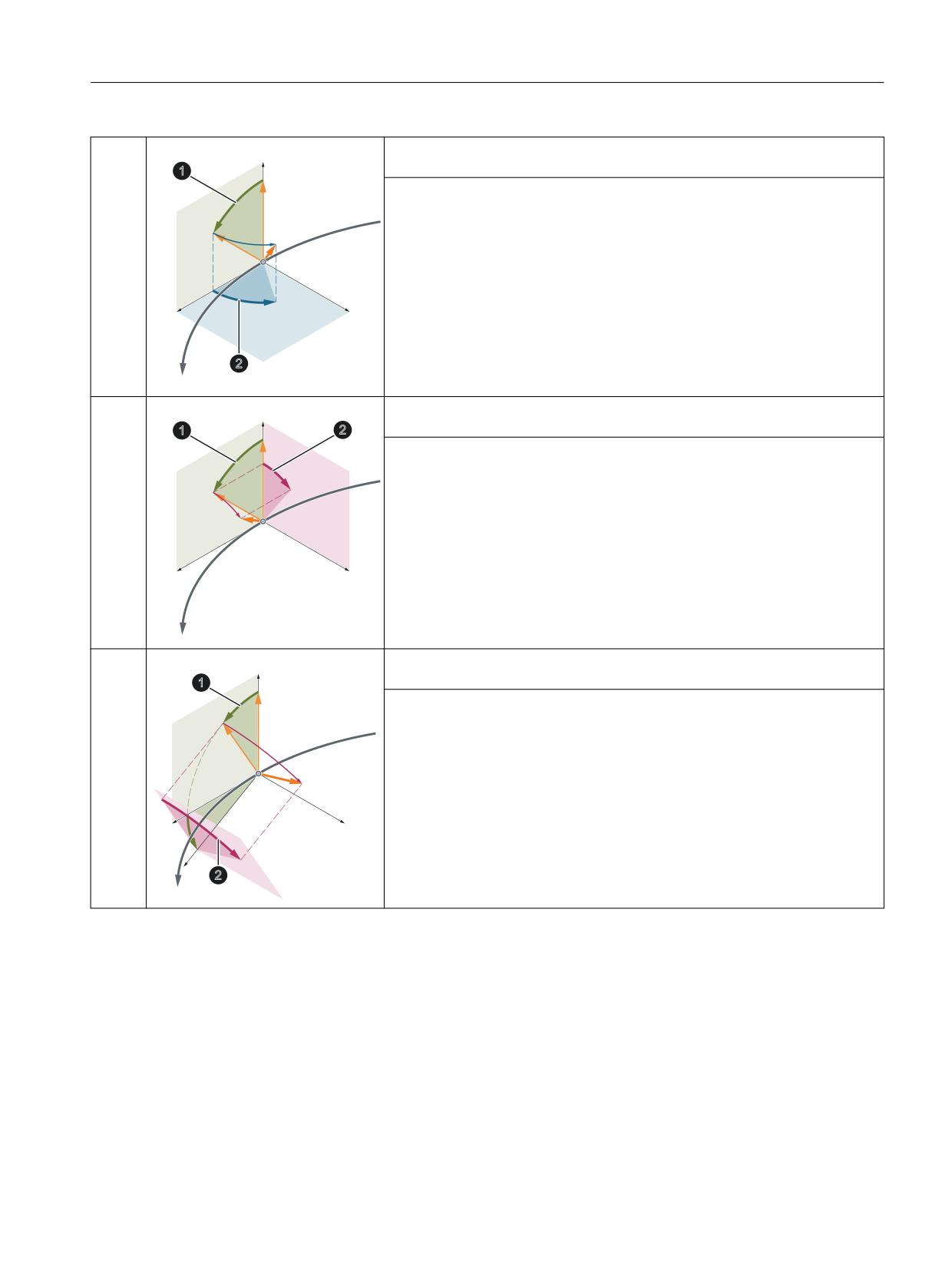
For path-relative orientation, the coordinate system is formed by the vectors path tangent T and programmed surface normal
vector N.
Note 1: Programming the surface normal vector N
• at the block start: A4=… B4=… C4=…
• at the block end: A5=… B5=… C5=…
Transformations
282
Function Manual, 10/2020, 6FC5397-5GP40-0BA1
Orientation transformations
6.7 Orientation
xx0x
ൺ
1st rotation LEAD: Rotation of the orientation vector O around the path normal
)
1
ൺ
vector BN ⇒ O'
2
/($'
2nd rotation TILT: Rotation of the new orientation vector O' around the sur-
face normal vector FN ⇒ O''
ൺ
2ಿ
ൺ
2ೀ
7&3
ൺ
ൺ
%7
%1
%
7,/7
xx1x
ൺ
1st rotation LEAD: Rotation of the orientation vector O around the path normal
)1
ൺ
vector BN ⇒ O'
2
/($'
7,/7
2nd rotation TILT: Rotation of the new orientation vector O' around the path
tangent vector BT ⇒ O''
ൺ
2ಿ
ൺ
2ೀ
7&3
ൺ
ൺ
%7
%1
%
xx2x
ൺ
1st rotation LEAD: Rotation of the orientation vector O and the path tangent
)
1
ൺ
vector BT around the path normal vector BN ⇒ O' and B'T
2
/($'
2nd rotation TILT: Rotation of the new orientation vector O' around the new
ൺ
2ಿ
path tangent vector B'T ⇒ O''
ൺ
2ೀ
7&3
ൺ
ൺ
%7
%1
ൺ
%ಿ7
%
7,/7
Transformations
Function Manual, 10/2020, 6FC5397-5GP40-0BA1
283
Orientation transformations
6.7 Orientation
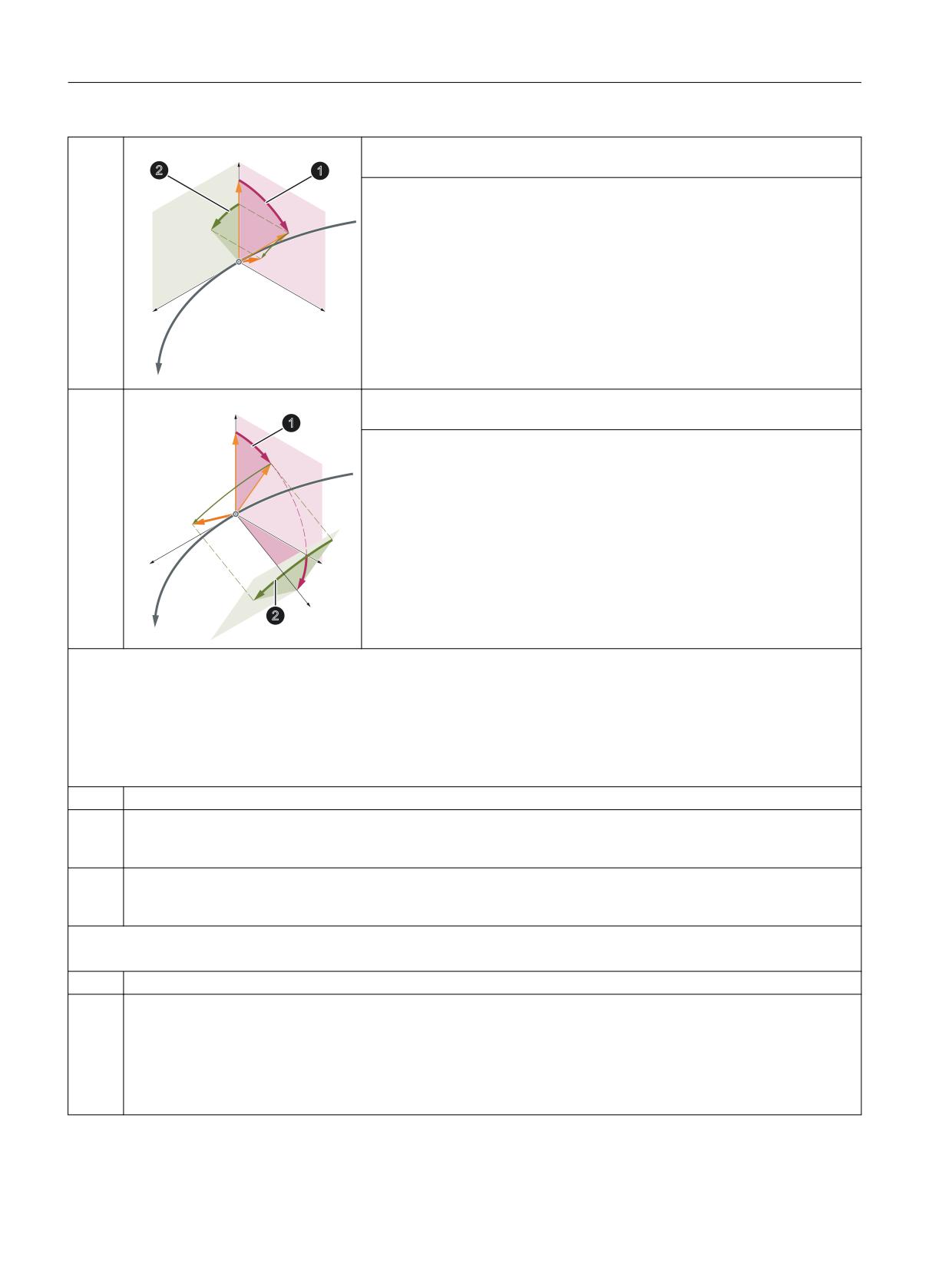
xx3x
ൺ
1st rotation TILT: Rotation of the new orientation vector O around the path
)
1
ൺ
tangent vector BT ⇒ O'
2
/($'
7,/7
2nd rotation LEAD: Rotation of the new orientation vector O' around the path
normal vector BN ⇒ O"
ൺ
2ಿ
ൺ
2ೀ
7&3
ൺ
ൺ
%7
%1
%
xx4x
ൺ
1st rotation TILT: Rotation of the orientation vector O and the path normal
)1
ൺ
vector BN around the path tangent vector BT ⇒ O' and B'N
2
7,/7
2nd rotation LEAD: Rotation of the new orientation vector O' around the new
ൺ
2ಿ
path normal vector B'N ⇒ O"
ൺ
2ೀ
7&3
ൺ
ൺ
%7
%1
ൺ
%ಿ1
%
/($'
Hundreds digit
(Activation and definition of the direction of the lift motion for reorientation during an active ORIPATH)
Note
A programmed retraction/lift motion is only executed, for:
• Once digit == 1 AND
• Length of the lift vector ≠ 0.0
x0xx
No lift motion is executed.
x1xx
Lift motion is executed in the direction of the programmed lift vector in the toolcoordinate system. The lift vector
refers to the coordinate system defined by the actual tool direction (z coordinate) and the orientation change (x
coordinate).
x2xx
Lift motion is executed in the direction of the programmed lift vector in the workpiececoordinate system. The lift
vector refers to the coordinate system that is defined by the active plane (z coordinate is the surface normal vector of
the active plane) and the orientation change (x coordinate).
Thousands digit
(Behavior of the path-relative orientation in the activation/deactivation blocks of the tool offset)
0xxx
The path-relative orientation is also maintained in activation or deactivation blocks of the tool offset.
1xxx
The path-relative orientation is not maintained in activation or deactivation blocks of the tool offset.
Note
The tool orientation normally remains constant in the activation or deactivation blocks of the tool offset. However, in
these blocks it is permitted to program a tool orientation, which is then traversed through in these blocks. However,
programming the orientation in these blocks is only possible with vectors; it is not permitted to program rotary axis
positions.
Transformations
284
Function Manual, 10/2020, 6FC5397-5GP40-0BA1
Orientation transformations
6.7 Orientation
Address names for the lift vector components
The address names for the lift vector components are defined using machine data:
MD10624 $MN_ORIPATH_LIFT_VECTOR_TAB[ <vector component> ] = <name>
Example with standard data
Machine data
$MN_ORIPATH_LIFT_VECTOR_TAB[ 0 ] = "A8" ; x coordinate
$MN_ORIPATH_LIFT_VECTOR_TAB[ 1 ] = "B8" ; y coordinate
$MN_ORIPATH_LIFT_VECTOR_TAB[ 2 ] = "C8" ; z coordinate
Programming
ORIPATHS A8=X_KOORD B8=Y_KOORD C8=Z_KOORD
Note
Naming convention
The rules defined by MD20080 $MC_AXCONF_CHANAX_NAME_TAB should be complied with
for axis identifiers.
Address names for the safety factor for orientation change
Normally the retracting movement is performed simultaneously to the orientation change. The
address name for safety factor R can be defined using machine data:
MD10626 $MN_ORIPATH_LIFT_FACTOR_NAME = "<name>"
If safety factor R is greater than 0.0, then the orientation is only changed if the tool is traversed
by safety clearance S in the direction of the lift vector. Safety clearance S is calculated as follows:
S = R * lift vector amount; definition range of factor R: 0 ≤ R < 1
Example with standard data
Machine data
$MN_ORIPATH_LIFT_FACTOR_NAME = "ORIPLF"
Programming
ORIPATHS A8=X_KOORD B8=Y_KOORD C8=Z_KOORD
; lift vector
ORIPLF=0.1
; safety clearance = 0.1 * lift vector amount (A8,
B8, C8)
Note
Naming convention
The rules defined by MD20080 $MC_AXCONF_CHANAX_NAME_TAB should be complied with
for axis identifiers.
Transformations
Function Manual, 10/2020, 6FC5397-5GP40-0BA1
285
Orientation transformations
6.7 Orientation
Parameterization: Setting data SD42670 (path section to the orientation smoothing)
Using the setting data, a path section is specified, within which, for a tool orientation step at a
block transition, it is possible to deviate from the programmed orientation path in order to
smooth the orientation path. If this path section is set too low, then it is possible that the path
velocity must be significantly reduced.
SD42670 $SC_ORIPATH_SMOOTH_DIST = <path length>
Response for path length 0.0
If a value of 0.0 is set as path length, then a dedicated intermediate block is inserted if necessary
to smooth the orientation path. The path is maintained until the orientation change was
executed in the intermediate block. However, the orientation change is then only performed
with continuous acceleration when ORIPATHS is active. Otherwise, from the start to the end
orientation, the orientation change is realized using linear large circle interpolation.
The tool can be lifted while the orientation axes are traversed to execute the orientation change.
The lift motion is activated via the hundreds digit of MD21094 $MC_ORIPATH_MODE (see the
paragraph above: "Parameterization: Machine data" > "Setting for path-relevant orientation").
The direction and path length of the lift motion is defined by the programmed lift vector (see
paragraph above: "Parameterization: Machine data" > "Address names for the lift vector
components"). If the length of this vector is exactly zero, no retracting movement is executed.
Normally the retracting movement is performed simultaneously to the orientation change.
However, a "Safety clearance" can also be programmed (see paragraph above:
"Parameterization: Machine data" > "Address names for the safety factor for orientation change")
Parameterization: Setting data SD42672 (tolerance for orientation smoothing)
If just the path and the path velocity are continuous at a block transition but not the path
acceleration (e.g. tangential transition, straight line/circle), then regarding the orientation, only
the orientation path is continuous, not the orientation change. This results in a generally
undesirable velocity step in the orientation axes. In the setting data, a tolerance window can be
parameterized; within this tolerance window it is permissible that the traversed orientation path
deviates from the programmed orientation path in order to smooth the orientation path.
SD42672 $SC_ORIPATH_SMOOTH_TOL = <tolerance>
This type of orientation smoothing is only executed if the following applies:
• ORIPATHS is active AND
• SD42672 $SC_ORIPATH_SMOOTH_TOL > 0.0
Path-relative interpolation of the rotation (ORIROTC)
For 6-axis transformations, in addition to the path-relative interpolation of all of the
components of the tool orientation (rotation around each of the three axes of rotation),
using ORIROTC it is possible that only the rotation of the tool around the orientation vector
relative to the path tangent is interpolated.
The orientation vector can still be programmed with direction components or via Euler or RPY
angle - and the interpolation type defined using ORIVECT, ORIAXES, ORICONxx, ORICURVE
(see Chapter "Rotations of orientation vector (Page 307)").
Transformations
286
Function Manual, 10/2020, 6FC5397-5GP40-0BA1
Orientation transformations
6.7 Orientation
6.7.9
Programming of orientation polynominals
Function
Orientation polynomials and even axis polynomials can be programmed with different types of
polynomials regardless of the type of polynomial interpolation currently active. This can be
applied to:
• Linear interpolation with G command G01
• Polynomial interpolation with G command TERMINAL
• Circular interpolation with G command G02, G03 or CIP
• Involute interpolation with G command INVCW or INVCCW
This enables a number of polynomials to be programmed for one contour at the same time.
Note
For additional information about programming axis polynomials with PO[X], PO[Y], PO[Z] and
orientation polynomials such as PO[PHI], PO[PSI], PO[THT] and PO[XH], PO[YH], PO[ZH], see:
Further information
"NC Programming" Programming Manual
Two different types of orientation polynomials are defined:
• Polynomials for angles with reference to the plane defined by the start and end orientation
(type 1 orientation polynomials)
• Polynomials for coordinates in space of a reference point on the tool (type 2 orientation
polynomials)
Type 1 polynomials
Orientation polynomials of type 1 are polynomials for angles
PO[PHI]:
Angle in the plane between start and end orientation
PO[PSI]:
Angle describing the tilt of the orientation from the plane between start and
end orientation
Type 2 polynomials
Orientation polynomials of type 2 are polynomials for coordinates
PO[XH]:
x coordinate of the reference point on the tool
PO[YH]:
y coordinate of the reference point on the tool
PO[ZH]:
z coordinate of the reference point on the tool
Transformations
Function Manual, 10/2020, 6FC5397-5GP40-0BA1
287
Orientation transformations
6.7 Orientation
Polynomials for angle of rotation and rotation vectors
For 6-axis transformations, the rotation of the tool around itself can be programmed for tool
orientation. This rotation of a third rotary axis is described either by an angle of rotation or by a
rotation vector, which is perpendicular to the tool direction in the plane.
In addition, a polynomial for rotation with PO[THT} of the orientation vector can be
programmed in these three cases. This is always possible if the kinematic transformation
applied, supports rotary angles.
Angle of rotation with ORIPATH and ORIPATHS
With orientation interpolation relative to the path with ORIPATH or ORIPATHS, the additional
rotation can be programmed with the angle THETA=<...>. In addition, for this angle of
rotation, with PO[THT]=(...) As a maximum, 5th degree polynomial angles can be
programmed.
The 3 possible angles, i.e. lead angle, tilt angle and angle of rotation, have the following
meaning with respect to the rotation effect:
LEAD: Angle relative to the surface normal vector in the plane put up by the path tangent and
the surface normal vector.
TILT:
Rotation of orientation in the z direction or rotation about the path tangent.
THETA: Rotation around the tool direction. This is only possible when the tool orientation has
a total of 3 degrees of freedom (see Section "Extension of the generic transformation
to 6 axes (Page 332)").
How the angles LEAD and TILT are to be interpreted, can be set with the following machine data:
MD21094 $MC_ORIPATH_MODE (setting for path relative orientation ORIPATH)
In addition to the constant angles programmed with LEAD and TILT, polynomials can be
programmed for lead angle and tilt angle. The polynomials are programmed using the angles
PHI and PSI:
PO[PHI]=(a2,a3,a Polynomial for the LEAD angle
4,a5):
PO[PSI]=(b2,b3,b Polynomial for the TILT angle
4,b5):
For both angles, as a maximum, 5th degree polynomial angles can be programmed. The angle
values at the block end are programmed with the NC addresses LEAD=<...> or TILT=<...>.
The higher polynomial coefficients, which are zero, can be omitted when programming. For
example PO[PHI] = (a2) programs a parabola for the lead angle LEAD.
Rotations of rotation vectors with ORIROTC
The rotation vector is interpolated relative to the path tangent with an offset that can be
programmed using the THETA angle.
Transformations
288
Function Manual, 10/2020, 6FC5397-5GP40-0BA1
Orientation transformations
6.7 Orientation
For the offset angle, with PO[THT]=(c2,c3,c4,c5), as a maximum, a 5th degree
polynomial angle can be programmed.
Note
If ORIAXES is active, i.e. the tool orientation is interpolated via axis interpolation, the orientation
of the rotation vector relative to the path is only fulfilled at the end of the block.
For further information on programming, see:
Further information
"NC Programming" Programming Manual
Boundary conditions
It is only useful to program orientation polynomials for specific interpolation types, which affect
both contour and orientation. A number of supplementary conditions must be met to avoid
illegal programming settings:
Orientation polynomials cannot be programmed,
• if ASPLINE, BSPLINE, CSPLINE spline interpolations are active.
Polynomials for type 1 orientation angles are possible for every type of interpolation except
spline interpolation, i.e. linear interpolation with rapid traverse G00 or with feedrate G01 and
polynomial POLY and circular/involute interpolation G02, G03, CIP, CT, INVCW and INVCCW.
In contrast, type 2 orientation polynomials are only possible if linear interpolation with rapid
traverse G00 or with feedrate G01 or polynomial interpolation POLY is active.
• if the orientation is interpolated using ORIAXES axis interpolation.
In this case, polynomials can be programmed directly with PO[A] and PO[B] for orientation
axes A and B.
If ORICURVE is active, the Cartesian components of the orientation vector are interpolated and
only type 2 orientation polynomials are possible. However, type 1 orientation polynomials are
not permitted.
Only type 1 orientation polynomials are possible for large circle interpolation and taper
interpolation with ORIVECT, ORIPLANE, ORICONxxx. However, type 2 orientation polynomials
are not permitted.
Alarms
An illegally programmed polynomial is signaled with the following alarms:
Alarm 14136:
Orientation polynomial is generally not allowed.
Alarm 14137:
Polynomials PO[PHI] and PO[PSI] are not permitted.
Alarm 14138:
Polynomials PO[XH], PO[YH], PO[ZH] are not permitted.
Alarm 14139:
Polynomial for angle of rotation PO[THT] is not permitted.
Transformations
Function Manual, 10/2020, 6FC5397-5GP40-0BA1
289

Orientation transformations
6.7 Orientation
6.7.10
System variable for tool orientation
The tool orientation can be read in various coordinate systems (BCS, WCS, SZS) via system
variables as well as also via OPI variables.
Tool orientation in BCS
System variable
Meaning
$AC_TOOLO_ACT[<i>]
; <i> = 1, 2, 3
i-th component of the vector of the actual reference
orientation
$AC_TOOLO_END[<i>]
; <i> = 1, 2, 3
i-th component of the vector of the end orientation
of the actual block
$AC_TOOLO_DIFF
Residual angle in degrees, i.e. this is the angle be-
tween vectors $AC_TOOLO_END[<i>] and $AC_TOO-
LO_ACT[<i>]
$VC_TOOLO[<i>]
; <i> = 1, 2, 3
i-th component of the vector of the actual orientation
$VC_TOOLO_DIFF
Angle in degrees between reference and actual value
orientation
$VC_TOOLO_STAT
Status variable for actual orientation
Indicates whether the actual orientation can be cal-
culated. The following values are possible:
0
Actual orientation can be calculated.
-1
Actual orientation cannot be calculated, as the
presently active transformation cannot calcu-
late these values in real time.
These system variables can always be read by the part program as well as in synchronized
actions. Write access operations are not permitted.
Note
The components of vectors $AC_TOOLO_ACT[<i>], $AC_TOOLO_END[<i>] and
$VC_TOOLO[<i>] of the orientation are scaled so that the orientation vector has the absolute
value of 1.
Rotation vector in the BCS
For a 6-axis kinematics, in addition to the orientation of the tool, there is also a rotation of the
tool, which can be changed.
System variable
Meaning
$P_TOOLROT[<i>]
; <i> = 1, 2, 3
i-th component of the actual rotation vector in the
NC program
$AC_TOOLR_ACT[<i>]
; <i> = 1, 2, 3
i-th component of the vector of the actual setpoint of
the orientation rotation
$AC_TOOLR_END[<i>]
; <i> = 1, 2, 3
i-th component of the vector of the setpoint of the
rotation at the end of the actual block
Transformations
290
Function Manual, 10/2020, 6FC5397-5GP40-0BA1
Orientation transformations
6.7 Orientation
System variable
Meaning
$AC_TOOLR_DIFF
Residual angle in degrees, i.e. this is the angle be-
tween vectors $AC_TOOLR_END[<i>] and
$AC_TOOLR_ACT[<i>]
$VC_TOOLR[<i>]
; <i> = 1, 2, 3
i-th component of the vector of the actual value of
the orientation rotation
$VC_TOOLR_DIFF
Angle in degrees between the setpoint and actual
value of the orientation rotation
$VC_TOOLR_STAT
Status variable for the actual value of the rotation
vector
Indicates whether the actual value of the rotation
vector can be calculated. The following values are
possible:
0
The actual value of the rotation vector can be
calculated.
-1
Actual value of the rotation vector cannot be
calculated, as the presently active transforma-
tion cannot calculate these values in real time.
Orientation and rotation of the tool in the various coordinate systems (BCS, WCS, SZS)
Tool orientation
System variable
Meaning
$P_TOOL_O[<i>,<j>]
; <i> =1, 2, 3
i-th component of the actual orientation vector in
the NC program in the coordinate system <j>
; <j> = 0, 1, 2
<j> = 0:
BCS
<j> = 1:
WCS
<j> = 2:
SZS
$AC_TOOL_O_ACT[<i>,< j>]
; <i> =1, 2, 3
i-th component of the actual orientation vector in
the coordinate system <j>
; <j> = 0, 1, 2
$AC_TOOL_O_END[<i>,< j>]
; <i> =1, 2, 3
i-th component of the end orientation of the actual
block in the coordinate system <j>
; <j> = 0, 1, 2
$AC_TOOL_O_DIFF[<j>]
; <j> = 0, 1, 2
Residual angle of the orientation vector in degrees in
various coordinate systems <j>
$VC_TOOL_O[<i>,<j>]
; <i> =1, 2, 3
i-th component of the vector of the actual orienta-
tion in various coordinate systems <j>
; <j> = 0, 1, 2
$VC_TOOL_O_DIFF[<j>]
; <j> = 0, 1, 2
Angle in degrees between reference and actual value
orientation in various coordinate systems <j>
Rotation vector (only for 6-axis kinematics)
System variable
$P_TOOL_R[<i>,<j>]
; <i> =1, 2, 3
i-th component of the actual rotation vector in the
NC program in the coordinate system <j>
; <j> = 0, 1, 2
<j> = 0:
BCS
<j> = 1:
WCS
<j> = 2:
SZS
Transformations
Function Manual, 10/2020, 6FC5397-5GP40-0BA1
291

Orientation transformations
6.8 Orientation axes
System variable
$AC_TOOL_R_ACT[<i>,<j>]
; <i> =1, 2, 3
i-th component of the actual rotation vector in the
coordinate system <j>
; <j> = 0, 1, 2
$AC_TOOL_R_END[<i>,<j>]
; <i> =1, 2, 3
i-th component of the rotation vector at the end of
the actual block in the coordinate system <j>
; <j> = 0, 1, 2
$AC_TOOL_R_DIFF[<j>]
; <j> = 0, 1, 2
Residual angle of the rotation vector in degrees in
various coordinate systems <j>
$VC_TOOL_R[<i>,<j>]
; <i> =1, 2, 3
i-th component of the actual value of the rotation
vector in various coordinate systems <j>
; <j> = 0, 1, 2
$VC_TOOL_R_DIFF[<j>]
; <j> = 0, 1, 2
Angle in degrees between reference and actual value
of the rotation vector in various coordinate systems
<j>
Boundary conditions
Not all transformations provide the actual value of the tool orientation in real time. In this case,
variables $VC_TOOLO[<i>] or VC_TOOL_O[<i>] and $VC_TOOLO_DIFF or $VC_TOOL_O_DIFF
cannot be calculated. The components of $VC_TOOLO[<i>] or $VC_TOOL_O[<i>] are all zero,
and status variable $VC_TOOLO_STAT supplies the value "-1". The same is true for the actual
values of the rotation vector $VC_TOOLR[<i>] or $VC_TOOL_R[<i>,<j>].
6.8
Orientation axes
6.8.1
Orientation axes - overview
Model for describing the change in orientation
The real-time transformation converts the Cartesian coordinates from the basic coordinate
system to the machine coordinate system. The Cartesian coordinates consist of the geometry
axes, which describe the working point, and the orientation axes, which describe the orientation
of the tool in space.
Real-time transformation
The Cartesian coordinates are converted from basic coordinate system to the machine
coordinate system by means of a real-time transformation.
These Cartesian coordinates comprise:
• Geometry axes
Geometry axes describe the working point.
• Orientation axes
Orientation axes describe the orientation of a tool in space.
Transformations
292
Function Manual, 10/2020, 6FC5397-5GP40-0BA1
Orientation transformations
6.8 Orientation axes
Orientation axes for transformations via kinematic chains
The rotary axes are defined via the kinematic chain as an element of the type "AXIS_ROT". For the
transformation, they are referenced with $NT_ROT_AX_NAME and are thus marked as
orientation axis:
• Definition of the machine kinematics (Page 228)
• Definition of the transformation (Page 231)
The system variable $NT_CNTRL (Page 47) defines further properties of orientation axes.
Orientation axes for conventional transformations
For conventional transformations, the orientation axes are defined by the transformation type
(Configuration of a machine for 5-axis transformation (Page 246))
6.8.2
Configuration of orientation axes
Directions of rotation
The orientation axes are defined by machine data that describe the directions around which the
orientation angles are to rotate and specify the rotating sequence. The directions are defined by
the axes of the reference system.
The directions around which axes are rotated are defined by the axes of the reference system.
The reference system is defined by ORIMKS and ORIWKS commands:
• ORIMKS : Reference system = Basic coordinate system
• ORIWKS: Reference system = Workpiece coordinate system
Order of rotation
The order of rotation for the orientation axes is defined by the following machine data:
MD21120 $MC_ORIAX_TURN_TAB_1[0..2] (definition of reference axes for ORI axes)
1. First rotation around the axis of the reference system, defined in the following machine data:
MD21120 $MC_ORIAX_TURN_TAB_1[0]
2. Second rotation around the axis of the reference system, defined in the following machine
data:
MD21120 $MC_ORIAX_TURN_TAB_1[1]
3. Third rotation around the axis of the reference system, defined in the following machine data:
MD21120 $MC_ORIAX_TURN_TAB_1[2]
Direction of the tool vector
The direction of the tool vector in the initial machine setting is defined in the following machine
data:
MD24580 $MC_TRAFO5_TOOL_VECTOR_1 (orientation vector direction) or
Transformations
Function Manual, 10/2020, 6FC5397-5GP40-0BA1
293
Orientation transformations
6.8 Orientation axes
MD24680 $MC_TRAFO5_TOOL_VECTOR_2 (orientation vector direction)
Assignment of the channel axes for transformations with kinematic chains
Via the machine data MD24585 $MC_TRAFO5_ORIAX_ASSIGN_TAB_1[0..2] (ORI/channel axis
assignment transformation 1), the up to 3 virtual orientation axes are assigned to the channel
and are set as input variables according to the machine data $NT_ROT_AX_NAME[n, 0...2] (axis
assignment for transformation n).
• $MC_TRAFO5_ORIAX_ASSIGN_TAB_n[0] = $NT_ROT_AX_NAME[n, 0]
• $MC_TRAFO5_ORIAX_ASSIGN_TAB_n[1] = $NT_ROT_AX_NAME[n, 1]
• $MC_TRAFO5_ORIAX_ASSIGN_TAB_n[2] = $NT_ROT_AX_NAME[n, 2]
Orientation transformation 1:
MD24585 $MC_TRAFO5_ORIAX_ASSIGN_TAB_1[n]
n = channel axis [0..2]
Orientation transformation 2:
MD24685 $MC_TRAFO5_ORIAX_ASSIGN_TAB_2[n]
n = channel axis [0..2]
Transformation [1..8]
$NT_ROT_AX_NAME[1, n]
n = axis index [0..2]
(axis assignment for transformation 1)
to
$NT_ROT_AX_NAME[8, n]
(axis assignment for transformation 8)
Assignment of the channel axes for conventional transformations
Machine data MD24585 $MC_TRAFO5_ORIAX_ASSIGN_TAB_1[0..2] (ORI/channel assignment
Transformation 1) are used to assign up to a total of 3 virtual orientation axes to the channel,
which are set as input variables in machine data $MC_TRAFO_AXES_IN_n[4..6] (axis assignment
for Transformation n).
For assigning channel axes to orientation axes, the following applies:
• $MC_TRAFO5_ORIAX_ASSIGN_TAB_n[0] = $MC_TRAFO_AXES_IN_n[4]
• $MC_TRAFO5_ORIAX_ASSIGN_TAB_n[1] = $MC_TRAFO_AXES_IN_n[5]
• $MC_TRAFO5_ORIAX_ASSIGN_TAB_n[2] = $MC_TRAFO_AXES_IN_n[6]
Orientation transformation 1:
MD24585 $MC_TRAFO5_ORIAX_ASSIGN_TAB_1[n]
n = channel axis [0..2]
Orientation transformation 2:
MD24685 $MC_TRAFO5_ORIAX_ASSIGN_TAB_2[n]
n = channel axis [0..2]
Transformation [1..4]
Transformations
294
Function Manual, 10/2020, 6FC5397-5GP40-0BA1
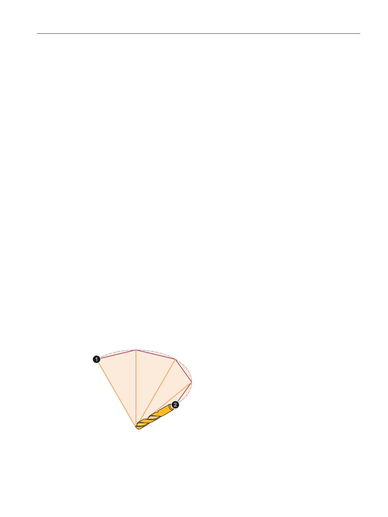
Orientation transformations
6.8 Orientation axes
MD24110 $MC_TRAFO5_AXES_IN_1[n] (axis assignment
n = channel axis [0..7]
for transformation)
to
MD24410 $MC_TRAFO5_AXES_IN_4[n] (axis assignment
for transformation 4)
Transformation [5..8]
MD24432 $MC_TRAFO5_AXES_IN_5[n] (axis assignment
n = channel axis [0..7]
for transformation 5)
to
MD24462 MC_TRAFO5_AXES_IN_8[n] (axis assignment for
transformation 8)
Example
For orientation axes, see Chapter "Example for orientation axes (Page 361)".
6.8.3
Interpolation of orientation axes
Interpolations
A 5-axis machine can apply any orientation to position the tool in relation to the workpiece. To
get from one orientation to another, intermediate positions must be interpolated, as these are
not specified in the NC program. These intermediate positions define the path from the start to
the end orientation.
Linear interpolation - ORIAXES
For linear interpolation from a starting position ① to an end orientation ②, the required rotary
axis motions are divided into equidistant sections. This results in a wall surface that is not flat
when using circumferential milling to create inclined walls, for example. By using sufficiently
small interpolation steps, an attempt is made to compensate for this effect.
Figure 6-26
Linear interpolation
Transformations
Function Manual, 10/2020, 6FC5397-5GP40-0BA1
295
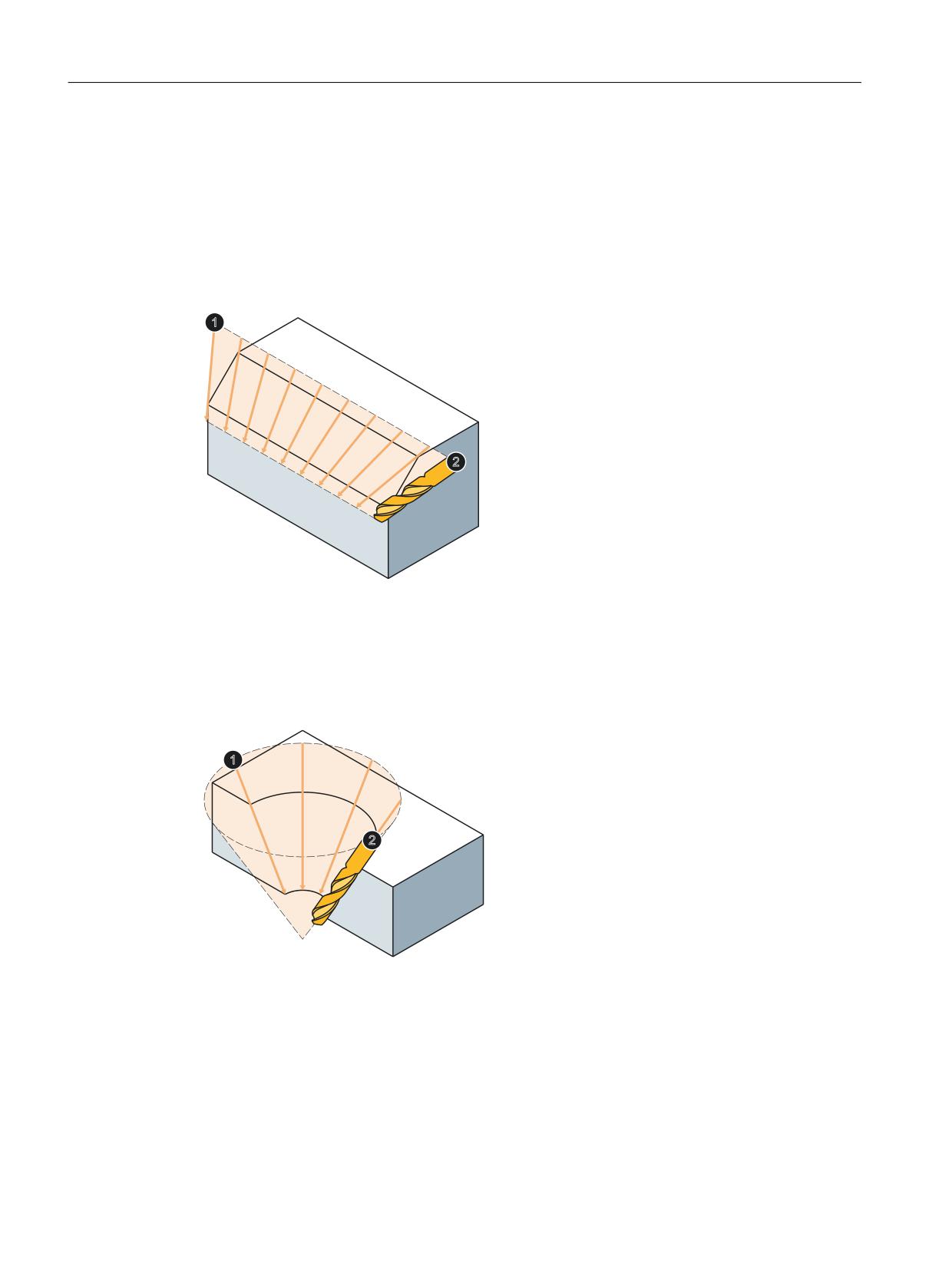
Orientation transformations
6.8 Orientation axes
Vector interpolation (large circle interpolation) - ORIVECT, ORIPLANE
For vector interpolation from a start orientation ① to an end orientation ②, the path is
interpolated in such a way that the orientation vector runs in a plane spanned by the start vector
and end vector.
The angle between the start vector and end vector is divided into equidistant steps at a constant
velocity. This kind of orientation interpolation can be used, for example, to enable precise
machining of sloping, flat walls in one block.
Figure 6-27
Vector interpolation
Cone surface interpolation - ORICON
For cone surface interpolation, the tool moves during reorientation on a programmable cone
surface located anywhere in space.
Figure 6-28
Cone surface interpolation
Transformations
296
Function Manual, 10/2020, 6FC5397-5GP40-0BA1
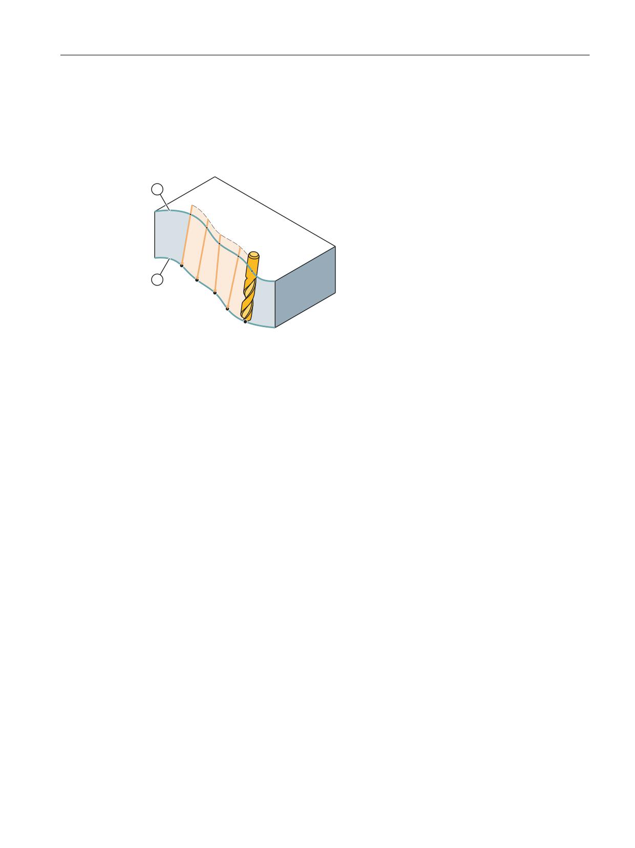
Orientation transformations
6.8 Orientation axes
Spline interpolation - ORICURVE
For spline interpolation, the motion of the orientation vector is described by the path of the tool
tip ① and the path of a second point on the tool ②. If, for example, an inclined surface is to be
created by circumferential milling, the surface on which the milling cutter is to move would be
defined by the two spline curves at the top and bottom ends of the tool (①, ②).
Figure 6-29
Spline interpolation
6.8.4
JOG mode
Preconditions
Orientation axes can only be traversed in the jog operating mode when the following
preconditions are satisfied:
• The orientation axis must be defined as such, that is, a value must be set in the following
machine data:
MD24585 $MC_TRAFO5_ORIAX_ASSIGN_TAB (ORI/channel axis assignment Transformation
1)
• A transformation must be active (TRAORI, TRAORI_DYN, TRAORI_STAT).
Traversing using traverse keys
When using the traverse keys to move an axis continuously or incrementally, it must be noted
that only one orientation axis can be moved at a time.
Alarm 20062 "Channel 1 axis 2 already active" is output if more than one orientation axis is
traversed.
Traversing using handwheels
More than one orientation axis can be moved simultaneously using handwheels.
Transformations
Function Manual, 10/2020, 6FC5397-5GP40-0BA1
297
Orientation transformations
6.8 Orientation axes
Velocity
When orientation axes are traversed manually, the channel-specific feedrate override switch or
the rapid traverse override switch in rapid traverse override applies.
Normally, velocities when traversing in the jog mode have always been derived from the
machine axis velocities. However, for geometry and orientation axes, there is not necessarily a
direct assignment to a particular machine axis. This is the reason that dedicated machine data
exist for geometry axes and orientation axes, which allow velocities to be separately specified:
• MD21150 $MC_JOG_VELO_RAPID_ORI[n] (conventional rapid traverse for ORI axes)
• MD21155 $MC_JOG_VELO_ORI[n] (conventional ORI axis velocity)
• MD21160 $MC_JOG_VELO_RAPID_GEO[n] (conventional rapid traverse for GEO axes)
• MD21165 $MC_JOG_VELO_GEO[n] (conventional GEO axis velocity)
Acceleration
The acceleration for orientation axes is set in machine data:
MD21170 $MC_ACCEL_ORI[n] (acceleration for orientation axes)
6.8.5
Programming for orientation transformation
The values can only be programmed in conjunction with an orientation transformation.
Programming of orientation
Orientation axes are programmed by means of axis names A2, B2 and C2.
Euler and RPY values are distinguished on the basis of G-group 50:
• ORIEULER:
Orientation programming on the basis of Euler angles (default)
• ORIRPY:
Orientation programming via RPY angles
• ORIVIRT1:
Orientation programming on the basis of virtual orientation axes (definition 1)
• ORIVIRT2:
Orientation programming on the basis of virtual orientation axes (definition 2)
The type of interpolation is distinguished on the basis of G-group 51:
• ORIAXES:
Orientation programming of linear interpolation of orientation axes or machine axes
• ORIVECT:
Orientation programming of large circle interpolation of orientation axes (interpolation of
the orientation vector)
Transformations
298
Function Manual, 10/2020, 6FC5397-5GP40-0BA1
Orientation transformations
6.8 Orientation axes
Machine data MD21102 $MC_ORI_DEF_WITH_G_CODE (definition of ORI axes via G command)
is used to specify whether MD21100 $MC_ORIENTATION_IS_EULER (angle definition for
orientation programming) is active (default) or G group 50.
The following four variants are available for programming orientation:
1. A, B, C:
Machine axis parameter designation
2. A2, B2, C2:
Angle programming of virtual axes
3. A3, B3, C3:
Vector component designation
4. LEAD, TILT:
Specification of lead and side angles with reference to path and surface
Further information
Programming Manual Fundamentals
Note
The four variants of orientation programming are mutually exclusive. If mixed values are
programmed, alarm 14130 or alarm 14131 is generated.
Exception:
For 6 axis kinematics with a 3rd degree of freedom for orientation, C2 may also be programmed
for variants 3 and 4. C2 in this case describes the rotation of the orientation vector about its own
axis.
Example
For orientation axes for kinematics with 6 or 5 transformed axes, see Section "Example for
orientation axes (Page 361)".
Interpolation type
The following machine data is used to specify which interpolation type is used:
MD21104 $MC_ORI_IPO_WITH_G_CODE (G command for orientation interpolation):
• ORIMKS or ORIWKS
• G group 51 with the commands ORIAXES or ORIVECT
- ORIAXES:
Linear interpolation of machine axes or orientation axes.
- ORIVECT:
Orientation is controlled by the orientation vector being swiveled in the plane spanned by
the start and end vectors (large circle interpolation). With 6 transformation axes a rotation
around the orientation vector is executed in addition to the swivel movement.
With ORIVECT the orientation axes are always traversed on the shortest possible path.
Transformations
Function Manual, 10/2020, 6FC5397-5GP40-0BA1
299
Orientation transformations
6.8 Orientation axes
Range of values
Value range for orientation axes:
•
180 degrees < A2 < 180 degrees
•
90 degrees < B2 < 90 degrees
•
180 degrees < C2 < 180 degrees
All possible rotations can be represented with this value range. Values outside the range are
normalized by the control system to within the range specified above.
Feedrate when programming ORIAXES
Feedrate for an orientation axis can be limited via the FL[ ] instruction (feed limit).
6.8.6
Programmable offset for kinematic chains
How the programmable offset works
The additional programmable offset for orientation axes acts in addition to the existing offset
and is specified when transformation is activated. Once transformation has been activated, it is
no longer possible to change this additive offset and no work offset will be applied to the
orientation axes in the event of an orientation transformation.
The programmable offset can be specified in two ways.
1. The offset is defined via the system variable $NT_ROT_AX_OFFSET (Page 39).
2. The offset is automatically transferred from the work offset for the orientation axes that is
active when the transformation is activated. This automatic transfer is configured via
machine data.
Programming the offset automatically
If the offset is automatically transferred from the currently active work offset of the orientation
axes, the effects of a work offset are always the same for the rotary axes with and without active
transformation. The offset from the work offset is automatically transferred via the system
variable $NT_ROT_OFSET_FROM_FRAME[n]
• If $NT_ROT_OFFSET_FROM_FRAME=1, the following applies:
The offsets for the orientation axes of the 5/6-axis transformation of the rotary axes, for
which the tool orientation is in the initial setting, are automatically defined. Thus, the offset
from an active work offset of the rotary axes, which is active as soon as the transformation
is switched on, is applied.
• If $NT_ROT_OFFSET_FROM_FRAME=0, then the following applies:
The transfer to the offset of the orientation axes is only performed if the work offsets are
maintained when the transformation is activated, i.e. MD10602
$MN_FRAME_GEOAX_CHANGE_MODE is > 0.
Transformations
300
Function Manual, 10/2020, 6FC5397-5GP40-0BA1
Orientation transformations
6.8 Orientation axes
6.8.7
Programmable offset for orientation axes (conventional)
How the programmable offset works
The additional programmable offset for orientation axes acts in addition to the existing offset
and is specified when transformation is activated. Once transformation has been activated, it is
no longer possible to change this additive offset and no zero offset will be applied to the
orientation axes in the event of an orientation transformation.
The programmable offset can be specified in two ways.
1. Direct programming of the offset with TRAORI() when transformation is activated.
2. Automatic transfer of the offset from the zero offset active for the orientation axes when
transformation is activated. This automatic transfer is configured via machine data.
Programming offset directly
When transformation is activated, the offset can be programmed directly as TRAORI(n, x,
y, z, a, b). The following parameters are available as an option:
n:
Number of transformation n = 1 or 2
x, y, z:
Components of the vector for the basic orientation of the tool (generic 5-axis
transformation only).
a, b:
Offset for rotary axes
These optional parameters can be omitted. However, if they are used for programming
purposes, the correct sequence must be observed. If for example only one rotary axis offset is to
be entered, TRAORI(,,,, a, b) is to be programmed.
For further information about programming, please refer to:
Further information
"NC Programming" Programming Manual
Programming the offset automatically
As the offset is transferred automatically from the currently active zero offset on the orientation
axes, the effects of zero offset on rotary axes are always the same, both with and without active
transformation. Automatic take-over of offset from zero offset is possible via machine data
MD24590 $MC_TRAFO5_ROT_OFFSET_FROM_FR_1 = TRUE (Offset of rotary transformation
axes from NPV) for the first machine data, or MD24690
$MC_TRAFO5_ROT_OFFSET_FROM_FR_2 = TRUE (Offset of rotary transformation axes from
NPV) for the second transformation in the channel.
Note
There is no difference between a zero offset on the orientation axes programmed during active
transformation and the previous offset.
If automatic transfer of offset has been activated and a rotary axis offset is programmed at the
same time, the programmed offset value takes priority.
Transformations
Function Manual, 10/2020, 6FC5397-5GP40-0BA1
301

Orientation transformations
6.8 Orientation axes
Orientable toolholder with additive offset
On an orientable toolholder, the offset for both rotary axes can be programmed with the system
variables $TC_CARR24 and $TC_CARR25. This rotary axis offset can be transferred automatically
from the zero offset effective at the time the orientable toolholder was activated.
Automatic transfer of offset from zero offset is made possible via the following machine data:
MD21186 $MC_TOCARR_ROT_OFFSET_FROM_FR = TRUE (offset of TOCARR rotary axes from
NPV)
Note
For more information about orientable toolholders, please see:
Further information
Function Manual Tools; Tool offset
6.8.8
Orientation transformation and orientable tool holders
Note
Orientation transformation and orientable tool holders can becombined.
The resulting orientation of the tool is produced by linking the orientation transformation and
the orientable tool holder.
6.8.9
Modulo display of orientation axes
Function
The positions of orientation axes can be displayed for the BCS and WCS display in a settable
modulo area. Whether the machine axes are linear or rotary is not relevant in this context. This
means that this display option can be enabled even for normal generic 5/6-axis transformation.
Requirements
• Orientation axes must be available. This is the case if an orientation transformation is active
(e.g. generic 5-/6-axis transformation).
• The following machine data must also be set for OEM transformations:
MD24585 $MC_TRAFO5_ORIAX_ASSIGN_TAB_1[0..2]
Parameterization
The modulo display of orientation axes is activated as follows:
MD21132 $MC_ORI_DISP_IS_MODULO[0...2] = TRUE
Transformations
302
Function Manual, 10/2020, 6FC5397-5GP40-0BA1
Orientation transformations
6.9 Orientation vectors
The modulo range is defined with the help of the following machine data:
• MD21134 $MC_ORI_MODULO_RANGE[0...2]
(Size of the modulo range for the display of the orientation axes)
• MD21136 $MC_ORI_MODULO_RANGE_START[0...2]
(Starting position of the modulo range for the display of the orientation axes)
Please note the following:
• The machine data become effective with NEWCONF.
• The machine data does not have any influence or effects on:
- any axis positions that can be programmed for these axes.
- The traversing movements of these axes.
- The display of the MCS values of these axes
6.9
Orientation vectors
6.9.1
Polynomial interpolation of orientation vectors
Programming of polynomials for axis motions
The rotary axes are normally subjected to linear interpolation in case of orientation changes with
the help of rotary axis interpolation. However, it is also possible to program the polynomials as
usual for the rotary axes. This allows a generally more homogeneous axis motion to be
produced.
Note
Further information about programming polynomial interpolation with POLY and on
interpolation of orientation vectors is given in:
Further information
"NC Programming" Programming Manual
A block with POLY is used to program polynomial interpolation. Whether the programmed
polynomials are then interpolated as polynomial, depends on whether the G command POLY is
active or not:
• The G command is not active: The programmed axis end points are traversed linearly.
• The G command is active: The programmed polynomials are interpolated as polynomials.
Transformations
Function Manual, 10/2020, 6FC5397-5GP40-0BA1
303
Orientation transformations
6.9 Orientation vectors
MD10674
Using machine data MD10674 $MN_PO_WITHOUT_POLY = FALSE
(polynomial can be programmed without G command POLY), it can be set as to whether the
following programming is possible:
• PO[...] or PO(...) is possible only if POLY is active, or
• PO[ ] or PO( ) polynomials are also possible without active G command POLY.
As default, MD10674: PO_WITHOUT_POLY = FALSE set and with MD10674
$MN_PO_WITHOUT_POLY = TRUE the following programming is always possible:
• PO[...] = (...), regardless of whether POLY is active or not.
Orientation polynomials can be programmed in conjunction with different interpolation types
and are described in Section "Programming of Orientation Polynomials".
POLYPATH:
In addition to the modal G command POLY, with the predefined subprogram
POLYPATH(argument), polynomial interpolation can be selectively activated for various axis
groups. The following arguments are allowed for the activation of polynomial interpolation
("AXES"):
For all path axes and supplementary axes
("VECT"):
For orientation axes
("AXES", "VECT"):
For path axes, supplementary axes and orientation axes
(without argument):
deactivates polynomial interpolation for all axis groups
Normally, the polynomial interpolation is activated for all axis groups.
Programming of orientation vectors
An orientation vector can be programmed in each block. If polynomials are programmed for the
orientation, the interpolated orientation vector is generally turned not in the plane between
start and end vector, but it can be rotated at random from this plane.
Orientation vectors can be programmed as follows:
1. Programming of rotary axis positions with A, B and C or with the actual rotary axis names.
2. Programming in Euler angle or RPY angle via A2, B2, C2
3. Programming of the direction vector via A3, B3, C3.
4. Programming using lead angle LEAD and tilt angle TILT.
Selection of type of interpolation
The type of interpolation of orientation axes is selected with G command of group 51 and is
independent of the programming type of the end vector:
• ORIAXES: Linear interpolation of the machine axes or using polynomials for active POLY or
• ORIVECT: Interpolation of the orientation vector using large circle interpolation
Transformations
304
Function Manual, 10/2020, 6FC5397-5GP40-0BA1
Orientation transformations
6.9 Orientation vectors
If ORIAXES is active, the interpolation of the rotary axis can also take place using polynomials
like polynomial interpolation of axes with POLY .
On the other hand, if ORIVECT is active, "normal" large circle interpolation is carried out
through linear interpolation of the angle of the orientation vector in the plane that is defined by
the start and end vector.
Polynomials for 2 angles
Additional programming of polynomials for 2 angles that span the start vector and end vector
can also be programmed as complex changes in orientation with ORIVECT .
The two PHI and PSI angles are specified in degrees.
POLY
Activation of polynomial interpolation for all axis groups.
POLYPATH ( )
Activation of polynomial interpolation for all axis groups. "AXES" and
"VECT" are possible groups.
The coefficients an and bn are specified in degrees.
PO[PHI]=(a2, a3, a4,
The angle PHI is interpolated according to PHI(u) = a0 + a1*u + a2*u2 +
a5)
a3*u3+ a4*u4 + a5*u5.
PO[PSI]=(b2, b3, b4,
The angle PHI is interpolated according to PSI(u) = b0 + b1*u + b2*u2 +
b5)
b3*u3+ b4*u4 + b5*u5.
PL
Length of the parameter interval where polynomials are defined. The
interval always starts at 0.
Theoretical value range for PL: 0.0001 ... 99999.9999.
The PL value applies to the block that contains it. PL = 1 is applied if no
PL value is programmed.
Rotation of the orientation vector
Changes in orientation are possible with ORIVECT independent of the type of end vector
programming. The following situations apply:
Example 1: Components of end vectors are programmed directly.
N... POLY A3=a B3=b C3=c PO[PHI] = (a2, a3, a4, a5) PO[PSI] = (b2, b3, b4, b5)
Example 2: The end vector is determined by the position of the rotary axes.
N... POLY Aa Bb Cc PO[PHI] = (a2, a3, a4, a5) PO[PSI] = (b2, b3, b4, b5)
The angle PHI describes the rotation of the orientation vector in the plane between start and end
vectors (large circle interpolation, see figure below). The orientation is interpolated exactly as in
Example 1.
Transformations
Function Manual, 10/2020, 6FC5397-5GP40-0BA1
305
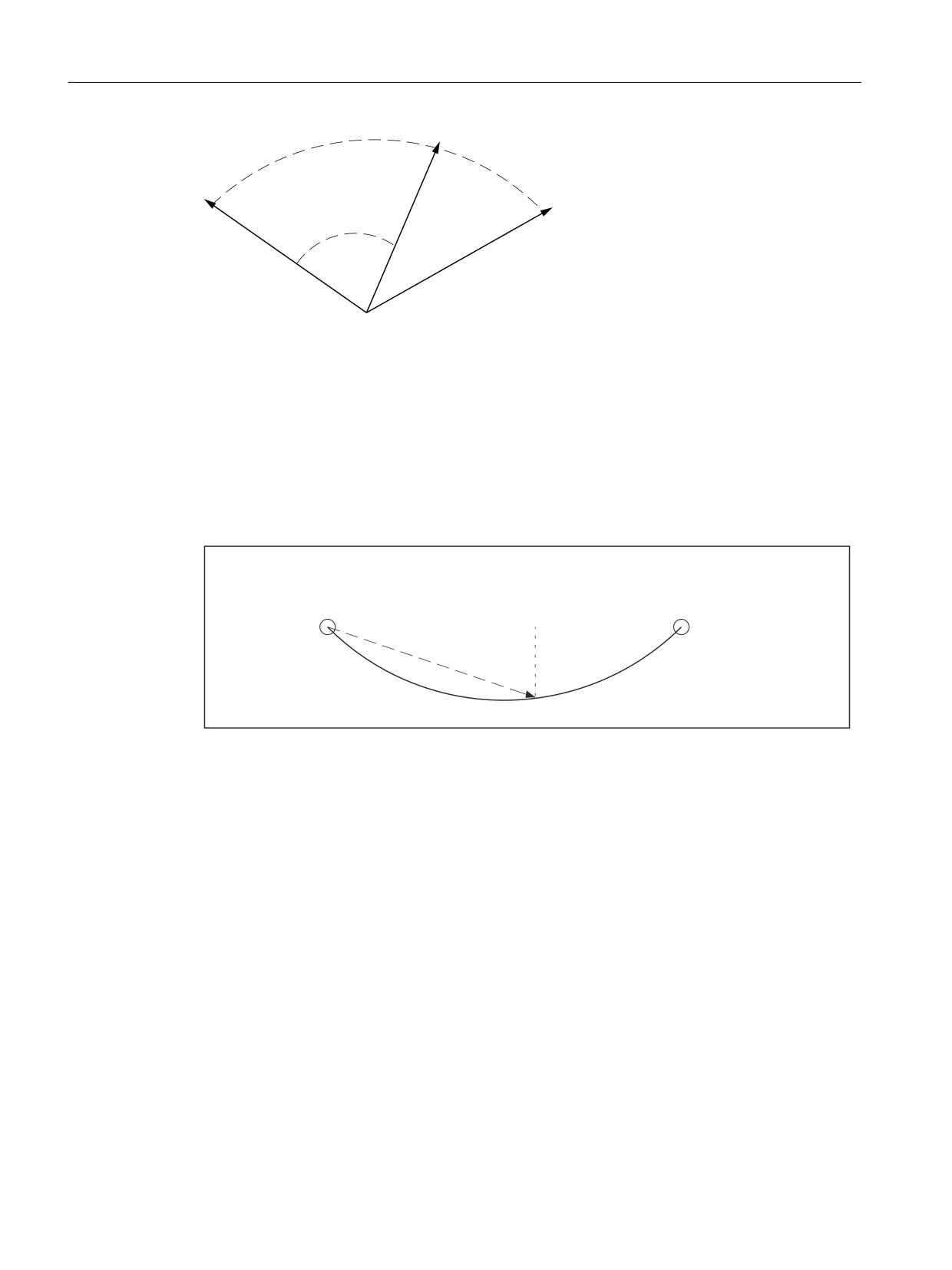
Orientation transformations
6.9 Orientation vectors
3+,
6WDUW YHFWRU
(QG YHFWRU
Figure 6-30
Rotation of the orientation vector in the plane between start and end vector
PHI and PSI angle
Programming of polynomials for the two angles PO[PHI] and PO[PSI] is always possible. Whether
the programmed polynomials are actually interpolated for PHI and PSI depends on:
• POLYPATH("VECT") and ORIVECT are active, then the polynomials will be interpolated.
• If POLYPATH("VECT") and ORIVECT are not active, the programmed orientation vectors
are traversed at the end of the block by a "normal" large circle interpolation. This means that
the polynomials for the two angles PHI and PSI are ignored in this case.
6WDUW
(QG
3+,
36,
Figure 6-31
Movement of the orientation vector in plan view
The angle PSI can be used to generate movements of the orientation vector perpendicular to
large circle interpolation plane (see previous figure).
Maximum polynomials of the 5th degree permitted
As a maximum, 5th degree polynomials can be programmed for the PHI and PSI angles. Here the
constants and linear coefficient are defined by the initial value or end value of the orientation
vector.
Higher degree coefficients can be omitted from the coefficient list (...,
) if these are all equal
to zero.
The length of the parameter interval in which the polynomials are defined can also be
programmed with PL.
Special situations
If no polynomial for angle PSI is programmed, the orientation vector is always interpolated in
the plane defined by the start and end vector.
Transformations
306
Function Manual, 10/2020, 6FC5397-5GP40-0BA1
Orientation transformations
6.9 Orientation vectors
The PHI angle in this plane is interpolated according to the programmed polynomial for PHI. As
a result the orientation vector moves through a "normal" large circle interpolation in the plane
between the start and end vector and the movement is more or less irregular depending on the
programmed polynomial.
In this way, the velocity and acceleration curve of the orientation axes can be influenced within
a block, for example.
Note
Further information on polynomial interpolation for axis motion and general programming is
given in:
Further information
"NC Programming" Programming Manual
Boundary conditions
Polynomial interpolation of orientation vectors is only possible for control variants in which the
following functions are included in the functional scope:
• Orientation transformation
• Polynomial interpolation
6.9.2
Rotations of orientation vector
Functionality
Changes in tool orientation are programmed by specifying an orientation vector in each block,
which is to be reached at the end of the block. The end orientation of each block can be
programmed in the following way:
1. Programming the vector directly, or
2. Programming the rotary axis positions.
The second option depends on the machine kinematics. Interpolation of the orientation vector
between the start and end values can also be modified by programming polynomials.
Programming of orientation directions
The following options are available for programming tool orientation:
1. Direct programming of rotary axis positions (the orientation vector is derived from machine
kinematics).
2. Programming in Euler angles via A2, B2, C2 (angle C2 is irrelevant).
3. Programming in RPY angles via A2, B2, C2.
4. Programming the direction vector via A3, B3, C3 (the length of the vector is irrelevant).
Transformations
Function Manual, 10/2020, 6FC5397-5GP40-0BA1
307
Orientation transformations
6.9 Orientation vectors
Switching between Euler and RPY angle programming can be selected via the following machine
data or via the G commands ORIEULER and ORIRPY :
MD21100 $MC_ORIENTATION_IS_EULER (angle definition for orientation programming)
Programming of orientation direction and rotation
While the direction of rotation is already defined when you program the orientation with RPY
angles, additional parameters are needed to specify the direction of rotation for the other
orientations:
1. Direct programming of the rotary axes
A supplementary rotary axis for direction of rotation has to be defined.
2. Programming in Euler angles via A2, B2, C2
Angle C2 must be programmed additionally. The complete orientation is thus defined,
including tool rotation.
3. Programming in RPY angles via A2, B2, C2
Additional settings are not required.
4. Programming of the direction vector via A3, B3, C3
The rotation angle is programmed with THETA=<value>.
Note
The following cases do not allow for a programmed rotation:
Multiple programming of the direction of rotation is not allowed and results in an alarm. If
the Euler angle C2 and the angle of rotation THETA are programmed simultaneously, the
programmed rotation is not executed.
If machine kinematics are such that the tool cannot be rotated, any programmed rotation is
ignored. This is the case with a normal 5-axis machine, for example.
Rotation of the orientation vector
The following options are available for interpolating rotation of the orientation vector by
programming the vector directly:
• Linear interpolation, i.e. the angle between the current rotation vector and the start vector
is a linear function of the path parameter.
• Non-linear due to additional programming of a polynomial for the angle of rotation q of
maximum 5th degree, in the form:
PO[THT] = (d2, d3, d4, d5)
Interpolation of the angle of rotation
Higher degree coefficients can be omitted from the coefficient list (...,
) if these are all equal
to zero.
In such cases, the end value of the angle and the constant and linear coefficient dn of the
polynomial cannot be directly programmed.
Linear coefficient dn is defined by the end angle qe, and is specified in degrees.
Transformations
308
Function Manual, 10/2020, 6FC5397-5GP40-0BA1
Orientation transformations
6.9 Orientation vectors
End angle q
e
is derived from the programming of the rotation vector.
Start angle qs is defined from the start value of the rotation vector, resulting from the end value
of the previous block. The constant coefficient of the polynomial is defined by the start angle of
the polynomial.
The rotation vector is always perpendicular to the actual tool orientation and forms the angle
THETA in conjunction with the basic rotation vector.
Note
When configuring the machine, the direction in space in which the rotation vector points at a
specific angle of rotation can be defined, when the tool is in the basic orientation.
Formula
In general, the angle of rotation is interpolated with a 5th degree polynomial:
θu=θs+d1u+d2u2+d3u3+d4u4+d5u5
(14)
For parameter interval 0 ... 1, this produces the following values for linear coefficients:
d1=θe -θs -d2-d3-d4-d5
(15)
Interpolation of the rotation vector
The programmed rotation vector can be interpolated in the following way, using modal G
commands:
• ORIROTA (orientation rotation absolute):
The angle of rotation THETA is interpreted with reference to an absolute direction in space.
The basic direction of rotation is defined by machine data.
• ORIROTR (orientation rotation relative):
Angle of rotation THETA is interpreted relative to the plane defined by the start and end
orientation.
• ORIROTT (orientation rotation tangential):
Angle of rotation THETA is interpreted relative to the change in orientation. This means the
rotation vector interpolation is tangential to the change in orientation for THETA=0.
This is only different to ORIROTR, if the change in orientation does not take place in one
plane. This is the case if, for the orientation, at least one polynomial was programmed for "tilt
angle" PSI. An additionally programmed angle of rotation THETA can then be used to
interpolate the rotation vector such that it always forms a specific angle referred to the
change in orientation.
Transformations
Function Manual, 10/2020, 6FC5397-5GP40-0BA1
309
Orientation transformations
6.9 Orientation vectors
Activating rotation
A rotation of the orientation vector is programmed with identifier THETA. The following
programming options are available:
THETA=<value>:
Programming an angle of rotation that is reached at the end of the
block.
THETA = qe
Programmed angle qe can be interpreted as absolute angle (G90 is
active) - as well as also relative angle (G91 is active incremental di-
mension).
THETA = AC(...)
Non-modal switchover to absolute dimensions
THETA = IC(...)
Non-modal switchover to incremental dimensions
PO[THT] = (...)
Programming a polynomial for rotation angle THETA.
Angle THETA is programmed in degrees.
Interpolation of the rotation vector is defined by modal G commands:
ORIROTA
Angle of rotation to an absolute direction of rotation
ORIROTR
Angle of rotation relative to the plane between the start and end
orientation
ORIROTT
Angle of rotation relative to the change of the orientation vector
tangential rotation vector to the orientation change
ORIROTC
Angle of rotation relative to the change of the orientation vector
tangential rotation vector to the path tangent
PL
Length of the parameter interval on which the polynomials are de-
fined. The interval always starts at 0. PL = 1 is active, if no PL value is
programmed.
These G commands define the reference direction of the angle of rotation. The meaning of the
programmed angle of rotation changes accordingly.
Supplementary conditions
The angle of rotation or rotation vector can only be programmed in all four modes if the
interpolation type ORIROTA is active.
1. Rotary axis positions
2. Euler angle via A2, B2, C2
3. RPY angle via A2, B2, C2
4. Direction vector via A3, B3, C3
If ORIROTR or ORIROTT is active, the angle of rotation can only be programmed directly with
THETA.
The other programming options must be excluded in this case, since the definition of an absolute
direction of rotation conflicts with the interpretation of the angle of rotation in these cases.
Possible programming combinations are monitored and an alarm is output if applicable.
A rotation can also be programmed in a separate block without an orientation change taking
place. In this case, ORIROTR and ORIROTT are irrelevant. In this case, the angle of rotation is
always interpreted with reference to the absolute direction (ORIROTA).
Transformations
310
Function Manual, 10/2020, 6FC5397-5GP40-0BA1
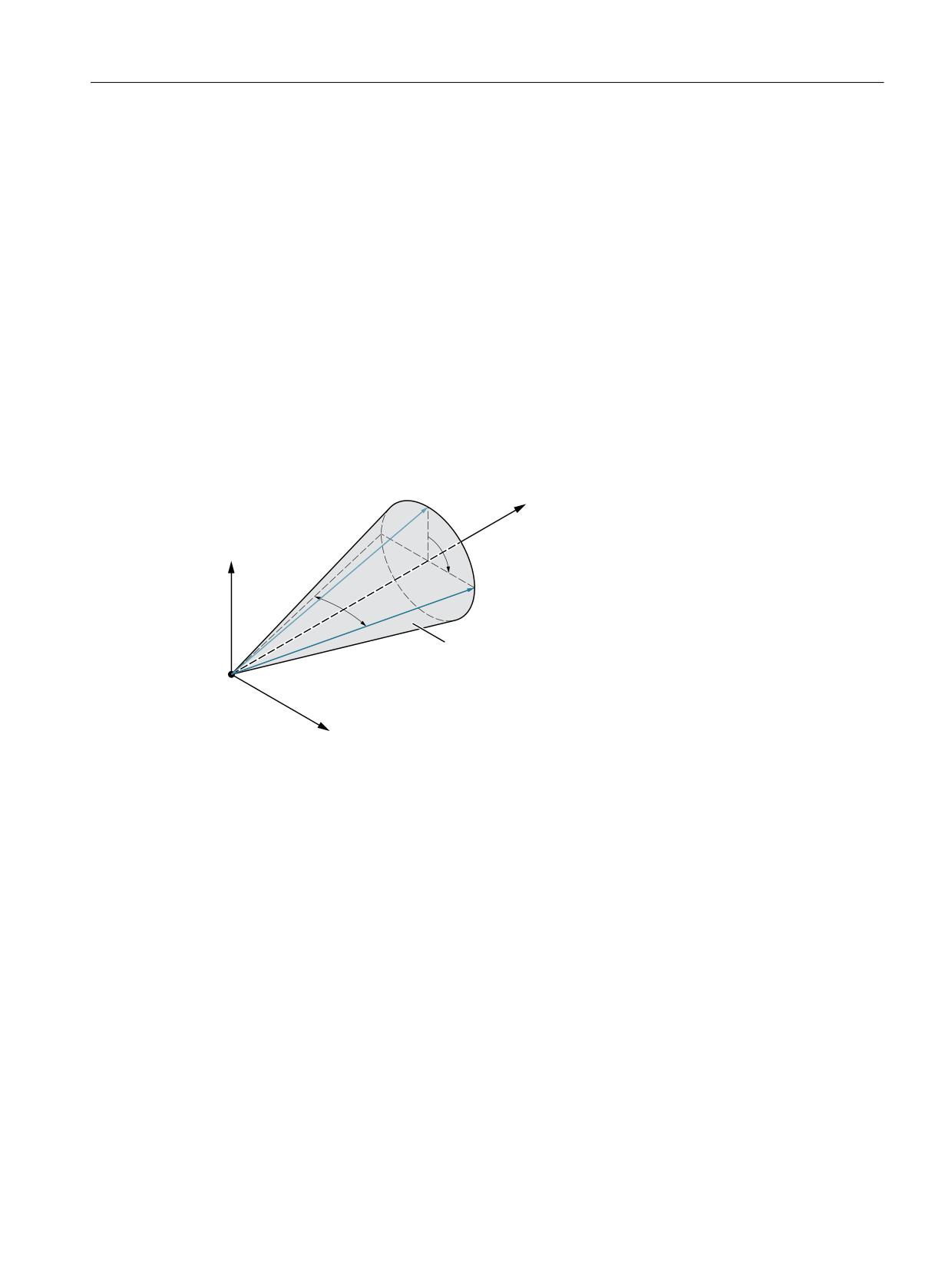
Orientation transformations
6.9 Orientation vectors
A programmable rotation of the orientation vector is only possible when an orientation
transformation (TRAORI) is active.
A programmed orientation rotation is only interpolated if the machine kinematics allow rotation
of the tool orientation (e.g. 6-axis machines).
6.9.3
Extended interpolation of orientation axes
Functionality
To execute a change in orientation along the peripheral surface of a cone located in space, it is
necessary to perform an extended interpolation of the orientation vector. The vector around
which the tool orientation is to be rotated must be known. The start and end orientation must
also be specified. The start orientation is given by the previous block and the en orientation must
either be programmed or defined by other conditions.
6WDUW YHFWRU
'LUHFWLRQ D[LV
3+,
(QG YHFWRU
36,
&RQLFDO VXUIDFH
Figure 6-32
Change in orientation of the peripheral surface of a cone located in space
Required definitions
Generally, the following data is required:
• The start orientation is defined by the end orientation of the previous block.
• The end orientation is defined either by specifying the vector (with A3, B3, C3), the Euler
angles or RPY angles (with A2, B2, C2) or by programming the positions of the rotary axis
(with A, B, C).
• The rotary axis of the taper is programmed as a (normalized) vector with A6, B6, C6.
Transformations
Function Manual, 10/2020, 6FC5397-5GP40-0BA1
311
Orientation transformations
6.9 Orientation vectors
• The opening angle of the cone is programmed degrees with the identifier (nutation angle).
The value range of this angle is limited to the interval between 0 degrees and 180 degrees.
The values 0 degrees and 180 degrees must not be programmed. If an angle is programmed
outside the valid interval, an alarm is generated.
In the special case where NUT = 90 degrees, the orientation vector in the plane is interpolated
perpendicular to the direction vector (large circle interpolation).
The sign of the programmed opening angle specifies whether the traversing angle is to be
greater or less than 180 degrees.
In order to define the cone, the direction vector or its opening angle must be programmed.
Both may not be specified at the same time.
• A further option is to program an intermediate orientation that lies between the start and
end orientation.
Programming
ORIPLANE
orientation interpolation in a plane: Interpolation in a plane
(large circle interpolation)
ORICONCW
orientation interpolation on a cone clockwise: Interpolation
on the peripheral surface of a cone in the clockwise direction
ORICONCCW
orientation interpolation on a cone counter clockwise: Inter-
polation on the peripheral surface of a cone in the counter-
clockwise direction.
Programming of the direction vector is carried out using the identifiers A6, B6, C6 and is
specified as a (normalized) vector.
Note
Programming of an end orientation is not absolutely necessary. If no end orientation is
specified, a full outside cone with 360 degrees is interpolated.
The opening angle of the taper is programmed with NUT= <angle>, where the angle is
specified in degrees.
Note
An end orientation must be specified. A complete outside cone with 360 degrees cannot be
interpolated in this way. The sign of the opening angle defines whether the traversing angle is
to be greater or less than 180 degrees.
The identifiers have the following meanings:
NUT = +...
Traverse angle smaller than or equal to 180 degrees
NUT = -...
Traverse angle greater than or equal to 180 degrees
A positive sign can be omitted when programming.
Transformations
312
Function Manual, 10/2020, 6FC5397-5GP40-0BA1
Orientation transformations
6.9 Orientation vectors
Settings for intermediate orientation
ORICONIO
orientation interpolation on a cone with intermediate orien-
tation: Interpolation on a conical peripheral surface with inter-
mediate orientation setting
If this G command is active, it is necessary to specify an intermediate orientation with A7, B7,
C7 which is specified as a (normalized) vector.
Note
Programming of the end orientation is absolutely necessary in this case.
The change in orientation and the direction of rotation is defined uniquely by the three
vectors Start, End and Intermediate orientation.
All three vectors must be different from each other. If the programmed intermediate orientation
is parallel to the start or end orientation, a linear large circle interpolation of the orientation is
executed in the plane that is defined by the start and end vector.
Angle of rotation and opening angle
The following may be programmed additionally for the angle of the cone:
PHI
angle of rotation for orientation about the direction axis
PSI
Opening angle of the cone
Besides this polynomials of the 5th degree (max.) can be programmed as follows:
PO[PHI] = (a2, a3, a4, a5) Constant and linear coefficients are defined by start and end orien-
tation respectively.
PO[PSI] = (b2, b3, b4, b5)
Further interpolation options
It is possible to interpolate the oreintation on a cone which connects tangentially to the previous
change of orientation. This orientation interpolation is achieved by programming the G
command ORICONTO.
ORICONTO
orientation interpolation on a cone with tangential orienta-
tion: Interpolation on a peripheral surface of the cone with
tangential transition
A further option for orientation interpolation is to describe the change in orientation through
the path of a 2nd contact point on the tool.
ORICURVE
orientation interpolation with a second curve: Interpolation of
orientation with specification of motion of two contact points
of the tool.
The coordinates for movement of the 2nd contact point of the tool must be specified. This
additional curve in space is programmed with XH, YH, ZH.
Besides the two end values, additional polynomials can be programmed in the following form:
Transformations
Function Manual, 10/2020, 6FC5397-5GP40-0BA1
313
Orientation transformations
6.9 Orientation vectors
PO[XH] = (xe, x2, x3, x4, x5): (xe, ye, ze) of the end point of the curve, and
PO[YH] = (ye, y2, y3, y4, y5): xi, yi, zi the coefficients of the polynomials
PO[ZH] = (ze, z2, z3, z4, z5): of the 5th degree maximum.
This type of interpolation can be used to program points (G1) or polynomials (POLY) for the two
curves in space.
Note
Circles or involutes are specificaly not allowed. It is also possible to activate a spindle
interpolation with BSPLINE. The programmed end points of both curves in space are then
interpreted as nodes.
Other types of splines (ASPLINE and CSPLINE) and the activation of a compressor function
(COMP...) are not permitted here.
General conditions
The extended interpolation of orientations requires that all necessary orientation
transformations be considered, since these belong to the functional scope.
Activation
A change in orientation on any peripheral surface of a cone in space is activated with the G
command of group 51 through extended interpolation of the orientation vector, using the
following commands:
ORIPLANE
Interpolation in a plane with specification of the end orienta-
tion (same as ORIVECT)
ORICONCW
Interpolation on a peripheral surface of a taper in clockwise
directionwith specification of the end orientation and taper
direction or opening angle of the cone.
ORICONCCW
Interpolation on the peripheral surface of a cone in the counter-
clockwise direction. Specification of the end orientation andt
cone direction or opening angle of the taper.
ORICONIO
Interpolation on a peripheral surface of a cone with specifica-
tion of end orientation and an intermediate orientation.
ORICONTO
Interpolation on a peripheral surface of a cone with tangential
transition and specification of end orientation.
ORICURVE
Interpolation of orientation with specification of motion of two
contact points of the tool.
ORIPATH
Tool orientation in relation to the path
ORIPATHS
Tool orientation in relation to the path, when, for example, a
kink in the orientation path, e.g. at a corner in the contour, is to
be smoothed (see Section "Path-relative orientation (ORIPATH,
ORIPATHS, ORIROTC) (Page 281)").
Transformations
314
Function Manual, 10/2020, 6FC5397-5GP40-0BA1
Orientation transformations
6.10 Online tool length offset
Examples
Various changes in orientation are programmed in the following program example:
Program code
Comment
N10 G1 X0 Y0 F5000
N20 TRAORI
; orientation transformation active.
N30 ORIVECT
; interpolate tool orientation as vector
N40 ORIPLANE
; select large circle interpolation.
N50 A3=0 B3=0 C3=1
N60 A3=0 B3=1 C3=1
; orientation in the Y/Z plane by 45
; degrees rotated, at the block end the
; orientation (0, 1 / (root of 2),
; 1 / (root of 2) is reached.
N70 ORICONCW
; the orientation vector is interpolated on a
; conical surface with direction
N80 A6=0 B6=0 C6=1 A3=1 B3=0 C3=1; (0, 0, 1) to the orientation
; (1 / (root of 2), 0, 1 / (root of 2)
; in the clockwise direction,
; the angle of rotation is 270 degrees.
; The tool orientation traverses a complete
N90 A6=0 B6=0 C6=1
; rotation on the same peripheral surface of the
cone
6.10
Online tool length offset
Functionality
Effective tool length can be changed in real time so that the length changes are also considered
for changes in orientation of the tool. The system variable $AA_TOFF[<geometry axis name>]
includes tool length compensations in 3-D according to the three tool directions.
None of the tool parameters are changed. The actual compensation is performed internally by
means of transformations using an orientable tool length compensation.
The number of active compensation directions must be the same as the number of active
geometry axes. All offsets can be active at the same time.
Transformations
Function Manual, 10/2020, 6FC5397-5GP40-0BA1
315

Orientation transformations
6.10 Online tool length offset
Application
The online tool length compensation function can be used for:
• Orientation transformations (TRAORI)
• Orientable tool carriers (TCARR)
Note
The online tool length offset is an option. This function is only practical in conjunction with
an active orientation transformation or an active orientable toolholder.
Further information
Function Manual Tools; Tool offset, orientable tool carriers
Block preparation
In the case of block preparation in run-in, the tool length offset currently active in the main run
is considered. In order to utilize the maximum permissible axis velocities as far as possible, it is
necessary to halt the block preparation with a stop preprocessing command (STOPRE) while a
tool offset is being generated.
The tool offset is always known at the time of run-in when the tool length offsets are not changed
after program start or if more blocks have been processed after changing the tool length offsets
than the IPO buffer can accommodate between run-in and main run. This ensures that correct
axis velocities are applied quickly.
The dimension for the difference between the currently active compensation in the interpolator
and the compensation that was active at the time of block preparation can be polled in the
system variable $AA_TOFF_PREP_DIFF[ ].
Note
Changing the effective tool length using online tool length offset produces changes in the
compensatory movements of the axes involved in the transformation in the event of changes in
orientation. The resulting velocities can be higher or lower depending on machine kinematics
and the current axis position.
MD21190 $MC_TOFF_MODE (operation of tool offset)
The following machine data can be used to set whether the content of the synchronization
variable $AA_TOFF[ ] is to be approached as an absolute value or whether an integrating
behavior is to take place:
MD21190 $MC_TOFF_MODE
The integrating behavior of $AA_TOFF[ ] allows 3D remote control. The integrated value is
available via the system variable $AA_TOFF_VAL[ ].
Transformations
316
Function Manual, 10/2020, 6FC5397-5GP40-0BA1

Orientation transformations
6.10 Online tool length offset
The following machine data and setting data are available for configuring online tool length
compensation:
Machine data / setting data
Meaning for online tool length offset
MD21190 $MC_TOFF_MODE
The contents of $AA_TOFF[ ] are traversed as an ab-
solute value or integrated
MD21194 $MC_TOFF_VELO (speed online tool
Speed of online tool length offset
offset)
MD21194 $MC_TOFF_ACCEL (acceleration on-
Acceleration of online tool length offset
line tool offset)
SD42970 $SC_TOFF_LIMIT (upper limit of offset
Upper limit of tool length offset value
value $AA_TOFF)
With the acceleration margin, 20% is reserved for the overlaid movement of online tool length
offset, which can be changed via the following machine data:
MD20610 $MC_ADD_MOVE_ACCEL_RESERVE(acceleration margin for overlaid movements)
Activation
The TOFFON instruction can be used to activate online tool length offset from the part program
for at least one tool direction, if the option is available. During activation an offset value can be
specified for the relevant direction of compensation and this is immediately traversed.
Example: TOFFON(Z, 25).
Repeated programming of the instruction TOFFON( ) with an offset causes the new offset to be
applied. The offset value is added to variables $AA_TOFF[ ] as an absolute value.
Note
For further information about programming plus programming examples, please see:
Further information
"NC Programming" Programming Manual
As long as online tool length offset is active, the VDI signal at the NC → PLC interface in the
following interface signal is set to 1:
DB21, ... DBX318.2 (TOFF active)
While a correction movement is active, the VDI → signal in the following interface signal is set
to 1:
DB21, ... DBX318.3 (TOFF movement active)
Reset
Compensation values can be reset with the TOFFOF( ) command. This instruction triggers a
preprocessing stop.
Accumulated tool length compensations are cleared and incorporated in the basic coordinate
system. The run-in is synchronized with the current position in main run. Since no axes can be
traversed here, the values of $AA_IM[ ] do not change. Only the values of the variables $AA_IW[ ]
Transformations
Function Manual, 10/2020, 6FC5397-5GP40-0BA1
317

Orientation transformations
6.10 Online tool length offset
and $AA_IB[ ] are changed. These variables now contain the deselected share of tool length
compensation.
Once "Online tool length offset" has been deselected for a tool direction, the value of system
variable $AA_TOFF[ ] or $AA_TOFF_VAL[ ] is zero for this tool direction. The following interface
signal is set to 0:
DB21, ... DBX318.2 (TOFF active)
Alarm 21670
An existing tool length offset must be deleted via TOFFOF( ) so that alarm 21670 "Channel %1
block %2, illegal change of tool direction active due to $AA_TOFF active" is suppressed:
• When the transformation is deactivated with TRAFOOF
• On switch-over from CP to PTP travel.
• If a tool length offset exists in the direction of the geometry axis during geometry
replacement.
• If a tool length offset is present during change of plane.
• When changing from axis-specific manual travel in the JOG mode to PTP as long as a tool
length offset is active. There is no switchover to PTP.
Mode change
Tool length compensation remains active even if the mode is changed and can be executed in
any mode.
If a tool length compensation is interpolated on account of $AA_TOFF[ ] during mode change,
the mode change cannot take place until the interpolation of the tool length compensation has
been completed. Alarm 16907 "Channel %1 action %2 <ALNX> possible only in stop state" is
issued.
Behavior with REF and block search
Tool length offset is not considered during reference point approach REF in JOG mode.
The instructions TOFFON( ) and TOFFOF( ) are not collected and output in an action block during
block search.
System variable
In the case of online tool length offset, the following system variables are available to the user:
System variable
Meaning for online tool length offset
$AA_TOFF[ ]
Position offset in the tool coordinate system
$AA_TOFF_VAL[ ]
Integrated position offset in the WCS
$AA_TOFF_LIMIT[ ]
Query whether the tool length offset value is close to the limit
$AA_TOFF_PREP_DIFF[ ]
Magnitude of the difference between the currently active value of
$AA_TOFF[ ] and the value prepared as the current motion block.
Transformations
318
Function Manual, 10/2020, 6FC5397-5GP40-0BA1
Orientation transformations
6.10 Online tool length offset
Further information
List Manual System Variables
Boundary conditions
The online tool length offset function is an option and is available during "generic 5-axis
transformation" by default and for "orientable toolholders".
If the tool is not perpendicular to the workpiece surface during processing or the contour
contains curvatures whose radius is smaller than the compensation dimension, deviations
compared to the actual offset surface are produced. It is not possible to produce exact offset
surfaces with one tool length compensation alone.
Transformations
Function Manual, 10/2020, 6FC5397-5GP40-0BA1
319