SINUMERIK 840D sl. Service - Functions. Manual (2018-2020) - page 67
M3: Coupled axes
10.2 Curve tables - 840D sl only
Overwriting curve tables
Curve tables that are not active in a master value coupling and are locked with CTABLOCK()
may be overwritten.
Deleting curve tables
Curve tables that are not active in a master value coupling and are locked with CTABLOCK()
may be overwritten.
10.2.4
Commissioning
10.2.4.1
Memory configuration
A defined storage space is available for the curve tables in the static and dynamic NC memory,
which is defined through the following machine data:
Static NC memory
MD18400 $MN_MM_NUM_CURVE_TABS
Defines the number of curve tables that can be stored in the
static NC memory.
MD18402 $MN_MM_NUM_CURVE_SEGMENTS
Defines the number of curve table segments that can be stored
in the static NC memory.
MD18403 $MN_MM_NUM_CURVE_SEG_LIN
Defines the maximum number of linear segments in the static
NC memory.
MD18404 $MN_MM_NUM_CURVE_POLYNOMS
Defines the number of curve table polynomes that can be stored
in the static NC memory.
Dynamic NC memory
MD18406 $MN_MM_NUM_CURVE_TABS_DRAM
Defines the number of curve tables that can be stored in the
dynamic NC memory.
MD18408 $MN_MM_NUM_CURVE_SEGNENTS_DRAM
Defines the number of curve table segments that can be stored
in the dynamic NC memory.
MD18409 $MN_MM_NUM_CURVE_SEG_LIN_DRAM
Defines the maximum number of linear segments in the dynam-
ic NC memory.
MD18410 $MN_MM_NUM_CURVE_POLYNOMS_DRAM
Defines the number of curve table polynomes that can be stored
in the dynamic NC memory.
Note
A curve table with linear segments can be stored efficiently in the memory only if:
MD18403 > 0 or MD18409 > 0
If no memory areas are created with this machine data, then the linear segments are stored
as polynomial segments.
Special functions
Function Manual, 12/2018, A5E40874099B AB
411
M3: Coupled axes
10.2 Curve tables - 840D sl only
10.2.4.2
Tool radius compensation
MD20900
Tool radius compensation can produce segments for which the following axis or leading axis
have no movement. A missing movement of the following axis does not normally represent
any problem. As against this, a missing movement of the leading axis requests a specification
as to how such discontinuities are to be handled, i.e., whether or not a curve table should be
generated in these cases. This specification is done in the machine data settings:
MD20900 $MC_CTAB_ENABLE_NO_LEADMOTION (curve tables with discontinuity of the
following axis)
Value
Description
0
No curve tables that contain a discontinuity in the following axis are produced. Alarm 10949
is output and program processing is aborted.
1
Curve tables with a discontinuity in the following axis can be generated. If a segment contains
a discontinuity in the following axis, Alarm 10955 is output but program processing is continued.
2
Curve tables with a discontinuity in the following axis can be created without an alarm being
output.
Note
In the case of a curve table that contains segments without leading axis movement (this means
that the following axis jumps at this point), the following axis can only make a jump within its
dynamic limits (max. velocity and max. acceleration). This means that there is always a
deviation from the programmed curve.
10.2.4.3
Specification of memory type
MD20905
If there is no memory specification while defining or deleting a curve table, the memory type
can be determined through the following machine data:
MD20905 $MC_CTAB_DEFAULT_MEMORY_TYPE (default memory type for curve tables)
Value
Description
0
Curve tabels are normally created in the static NC memory.
1
Curve tabels are normally created in the dynamic NC memory.
Special functions
412
Function Manual, 12/2018, A5E40874099B AB
M3: Coupled axes
10.2 Curve tables - 840D sl only
10.2.5
Programming
Definition
The following modal language commands work with curve tables: (The parameters are
explained at the end of the list of functions.)
● Beginning of definition of a curve table:
CTABDEF(following axis, leading axis, n, applim, memType)
● End of definition of a curve table:
CTABEND()
● Deleting curve table(s):
CTABDEL(n)
; curve table n
CTABDEL(n, m)
; [n < m], more than one in the range of numbers
; it is deleted in static "SRAM" and in dynamic "DRAM" of NC memory.
● CTABDEL(n, m, memType)
; Delete with memory specification:
Those curve tables with the numbers in the range, which are in the specified memory type,
will be deleted. All other curve tables are retained.
Delete all tables in a particular memory type:
CTABDEL(, , "DRAM")
CTABDEL(, , "SRAM")
CTABDEL()
; all in DRAM or
; all in SRAM:
; all, irrespective of memory type
● Read the following value for a master value
CTAB(master value, n, degrees, [following axis, lead axis])
● Read the master value for a following value
CTABINV(following value, approx. master value, n, degrees, [following axis, leading axis])
Special functions
Function Manual, 12/2018, A5E40874099B AB
413
M3: Coupled axes
10.2 Curve tables - 840D sl only
Access to curve table segments
● Read start value (following axis value) of a table segment
CTABSSV(leading value, n, degrees, [following axis, leading axis])
● Read end value (following axis value) of a table segment
CTABSEV(master value, n, degrees, [following axis, master axis])
Note
If curve table functions such as CTAB(), CTABINV(), CTABSSV() etc., in synchronous
actions are used, only main traverse variable, e.g. $AC_PARAM[ ... ] or $R[ ... ] is
permissible for the return value and the argument "degrees" of the function.
Example:
ID=1 WHEN TRUE DO $R1 = CTABSSV(10, 1, $R2)
or
ID=1 WHEN TRUE DO $AC_PARAM[1] = CTABSSV(10, 1, $AC_PARAM[2])
Enable/cancel blocking
The following functions can be used to enable or cancel deletion and overwrite blocks for parts.
programs.
● Enable deletion and overwrite block.
General form: CTABLOCK(n, m, memType)
● Cancel deletion and overwrite block.
CTABUNLOCK releases the tables locked with CTABLOCK. Tables involved in an active
coupling remain locked, i.e. they cannot be deleted. However, the CTABLOCK command is
cancelled, i.e. the table can be deleted as soon as the coupling is deactivated. It is not
necessary to call CTABUNLOCK again.
General form: CTABUNLOCK(n, m, memType)
Applications of the forms:
Curve table with number n
CTABLOCK(n)
Curve tables in the number range n to m.
CTABLOCK(n, m)
All curve tables, irrespective of memory type
CTABLOCK()
All curve tables in the specified memory type
CTABLOCK(, , memType)
Curve table with number n
CTABUNLOCK(n)
Curve tables in the number range n to m.
CTABUNLOCK(n, m)
Special functions
414
Function Manual, 12/2018, A5E40874099B AB
M3: Coupled axes
10.2 Curve tables - 840D sl only
All curve tables, irrespective of memory type
CTABUNLOCK()
All curve tables in the specified memory type
CTABUNLOCK(, , memType)
Other commands for calculating and differentiating between curve tables for applications for
diagnosing and optimizing the use of resources:
●
Number of defined tables irrespective of memory type
CTABNO()
●
Number of defined tables in SRAM or DRAM of NC memory
CTABNOMEM(memType)
●
Number of possible curve tables in memory memType.
CTABFNO(memType)
●
Table number of nth curve table.
General form: CTABID(n, memType)
Generates the table number of the nth curve table with memory type memType. CTABID(1,
memType) is used to read out the highest curve number (105) of the memory type specified.
CTABID(n)
Generates the table number of the nth curve table in the memory specified using the
following machine data:
MD20905 $MC_CTAB_DEFAULT_MEMORY_TYPE (default memory type for curve
tables)
CTABID(p)
Generates the ID (table number) of the curve table entered in the memory as the pth curve
table.
Note
If for example, the sequence is changed between consecutive calls of CTABID(), then
CTABID(n, ...) can be used to provide a different curve table than the one provided before
the change.
●
Indicates the block state of curve table number n.
CTABISLOCK(n)
●
Checks curve table number n.
CTABEXISTS(n)
●
Returns the memory in which curve table number n is stored.
CTABMEMTYP(n)
●
Returns the table periodicity.
CTABPERIOD(n)
●
Number of curve segments already used in memory memType.
CTABSEG(memType, segType)
●
Number of curve segments used in curve table number n
CTABSEGID(n, segType)
●
Number of still possible curve segments in memory memType.
CTABFSEG(memType, segType)
Special functions
Function Manual, 12/2018, A5E40874099B AB
415
M3: Coupled axes
10.2 Curve tables - 840D sl only
● Maximum number of possible curve segments in memory memType.
CTABMSEG(memType, segType)
● Number of polynomials already used in memory memType.
CTABPOL(memType)
● Number of curve polynomials used by curve table number n.
CTABPOLID(n)
● Number of still possible polynomials in memory memType.
CTABFPOL(n)
● Maximum number of possible polynomials in memory memType.
CTABMPOL(n)
Boundary values of curve tables
Behavior of the leading axis/following axes on the edges of the curve table:
● The value at the beginning of the curve table is read by a following axis.
CTABTSV(n, degrees, F axis), following value at the beginning of the curve table
● The value at the end of the curve table is read by a following axis.
CTABTEV(n, degrees, FAxis), following value at the end of the curve table
● The value at the beginning of the curve table is read by the leading axis.
CTABTSP(n, degrees, FAxis), master value at the beginning of the curve table
● The value at the end of the curve table is read by the leading axis.
CTABTEP(n, degrees, FAxis), master value at the end of the curve table
● Determine the value range of the following value.
CTABTMIN(n, FAxis), minimum following value of curve table
CTABTMAX(n, FAxis), maximum following value of the curve table
Parameter
● Following axis:
Name of axis via which the following axis is programmed in the definition.
● Leading axis:
Name of axis via which the leading axis is programmed.
● n, m
Numbers for curve tables.
Curve table numbers can be freely assigned. They are used exclusively to uniquely identify
a curve table.
In order to delete a curve table area using the command CTABDEL(n, m) must be greater
than n.
● p
Entry location (in memType memory area)
Special functions
416
Function Manual, 12/2018, A5E40874099B AB
M3: Coupled axes
10.2 Curve tables - 840D sl only
●
applim:
Behavior at the curve table edges.
-
0 non-periodic (table is processed only once, even for rotary axes).
–
1 periodic, modulo (the modulo value corresponds to the LA table values).
-
2 periodic, modulo (LA and FA are periodic).
●
Master value
Position value for which a following value is to be determined.
●
Slave value
Position value for which a master value is to be calculated.
●
aproxmastervalue
Position value that can be used to determine a unique master value in the case of an
ambiguous reversing function of the curve table.
●
degrees
Parameter in which the pitch of the table function is returned.
●
memType
Optional parameter for specifying memory type to be used n curve tables.
Possible values:
"SRAM" curve table is created in static NC memory.
"DSRAM" curve table is created in dynamic NC memory.
If an invalid type is entered, the value -2 is returned.
If the parameter is omitted, then the memory type set via the following machine data takes
effect:
MD20905 $MC_CTAB_DEFAULT_MEMORY_TYPE (default memory type for curve
tables)
●
segType
Optional parameter for entry of segment type
Possible values:
segType "L" linear segments
segType "P" Polynomial segments
Reference:
Programming Manual, Production Planning; Axis Couplings, Section: Curve tables (CTAB)
Restrictions
The following restrictions apply when programming:
● It is not permissible that the NC block generates a preprocessing stop.
● No discontinuities may occur in leading axis motion.
● Any block that contains a traverse instruction for the following axis must also include a
traverse for the leading axis.
● The direction of motion of the leading axis must not reverse at any point in the rule of motion,
i.e. the position of the leading axis must always be unique within the sequence of motions.
The programmed contour may not move perpendicular to the leading axis.
Special functions
Function Manual, 12/2018, A5E40874099B AB
417
M3: Coupled axes
10.2 Curve tables - 840D sl only
● Axis names from gantry axis groups cannot be used to define a table (only leading axis are
possible).
● Depending on the following machine data, jumps in the following axis may be tolerated if
a movement is missing in the leading axis.
MD20900 $MC_CTAB_ENABLE_NO_LEADMOTION (curve tables with discontinuity of the
following axis)
The other restrictions listed above still apply.
Axis assignment
Does not take effect until coupling is activated with curve table.
Note
The dynamic limit values of the motion commands for a curve table are not checked until
activation or interpolation.
Starting value
The first motion command in the definition of a curve table defines the starting value for the
leading and following value.
All instructions that cause a preprocessing stop must be hidden.
Example 1
Without tool radius compensation, without memory type
Program code
Comment
N100 CTABDEF(AX2, AX1, 3,0)
; start of the definition for the non-
; periodic curve table no. 3
N110 AX1=0 AX2=0
; 1st Motion instruction specifies the start value
; leading value: 0, Following value: 0
N110 AX1=20 AX2=0
; 1st Curve segment: Master value: 0...20,
; following value: Starting value …0
N120 AX1=100 AX2=6
; 2nd Curve segment: Master value: 20...100,
; following value: 0...6
N130 AX1=150 AX2=6
; 3rd Curve segment: Master value: 100...150,
; following value 6
N130 AX1=180 AX2=0
; 4th Curve segment: Master value: 150...180,
; following value: 6...0
N200 CTABEND
; end of the definition, the curve table
; is generated in its internal representation.
; the advance is reorganized to the status
; at the start of N100
Special functions
418
Function Manual, 12/2018, A5E40874099B AB
M3: Coupled axes
10.2 Curve tables - 840D sl only
Example 2
Example of a curve table with active tool radius compensation:
Prior to definition of a curve table with CTABDEF(), tool radius compensation must not be active;
otherwise alarm 10942 is generated. This means that tool radius compensation must be
activated within the definition of the curve table. Similarly, it must be deactivated again before
the end of the curve table definition, using CTABEND.
Program code
Comment
N10 CTABDEF(Y, X, 1, 0)
; start of the definition for the non-
; periodic curve table no. 1
N20 X0 Y0
N30 G41 X10 Y0
; tool radius compensation on
N40 X20 Y20
N50 X40 Y0
N60 X60 Y20
N70 X80 Y0
N80 G40 X90 Y0
; tool radius compensation off
N90 CTABEND
Tool radius compensation is activated in block N30; this causes the approach movement for
radius compensation to be made in this block. Similarly, the approach movement for
deactivation of the radius compensation is made in block N80.
Note
The value pairs between CTABDEF and CTABENDmust be specified for precisely the axis
names that have been programmed in CTABDEF as the leading axis name and following axis
name. In the case of programming errors, alarms or incorrect contours may be generated.
10.2.6
Access to table positions and table segments
Reading table positions
With the program commands CTAB and CTABINV the following value for a master value
(CTAB) can be read from the part program and from synchronous actions, or alternatively the
master value can be read off for a following value. The pitch value can be used to calculate
the speed of the following axis or leading axis at any position in the table.
Reading segment positions
Segment positions of a curve table for the value for the following axis can be read using the
CTABSSV and CTABSEV calls.
The language commands CTABSSV and CTABSEV generally provide the start and end values
of the internal segments of the curve tables for the following axis. These values only agree
with the programmed values of the curve tables if the programmed segments can be converted
Special functions
Function Manual, 12/2018, A5E40874099B AB
419
M3: Coupled axes
10.2 Curve tables - 840D sl only
1:1 to the internal segments of the curve table. This is always the case if only G1 blocks or axis
polynomials are used to define the curve tables and no other functions are active.
Programmed sections may under certain circumstances not be transformed unchanged into
internal curve segments if:
1. Circles or involutes are programmed
2. Chamfer or rounding is active (CHF, RND)
3. Smoothing with G643 is active
4. Compressor is active (COMPON, COMPCURV, COMPCAD)
5. Tool radius compensation is active for polynomial interpolation.
In these cases, the language commands CTABSSV and CTABSEV may not be used to query
the start and end points of the programmed segments.
CTABINV
When using the inversion function for the curve tables CTABINV, it must be noted that the
following value mapped to the leading value may not be unique.
Within a curve table, the following value can assume the same value for any number of master
value positions. In order to resolve this ambiguity, the program command CTABINV requires
a further parameter, in addition to the following value, which it uses to select the 'correct' master
value. CTABINV always returns the master value that is closest to this auxiliary parameter.
This auxiliary value can, for example, be the master value from the previous interpolator clock
cycle.
Note
Although the auxiliary parameter permits calculation of a unique result for the reversal function
of the curve table, it should be noted that numerical inaccuracies may give rise to contours,
which can cause the reversal function to produce results that deviate from those that would
be obtained in a calculation where the accuracy is unrestricted.
Optional parameters
The functions CTAB, CTABINV, CTABSSV and CTABSEV have optional parameters for the
leading and following axes. If one of these parameters is programmed, the master value and
following value are modified using the scaling factors of the relevant axes.
This is particularly important if axes have been configured with different length units (inch/
metric). If no optional parameters are programmed, the master value and following value are
treated as path positions in the conversion from external to internal representation. This means
that the values are multiplied according to the configured resolution (decimal places) and the
remaining decimal places are truncated.
Special functions
420
Function Manual, 12/2018, A5E40874099B AB
M3: Coupled axes
10.2 Curve tables - 840D sl only
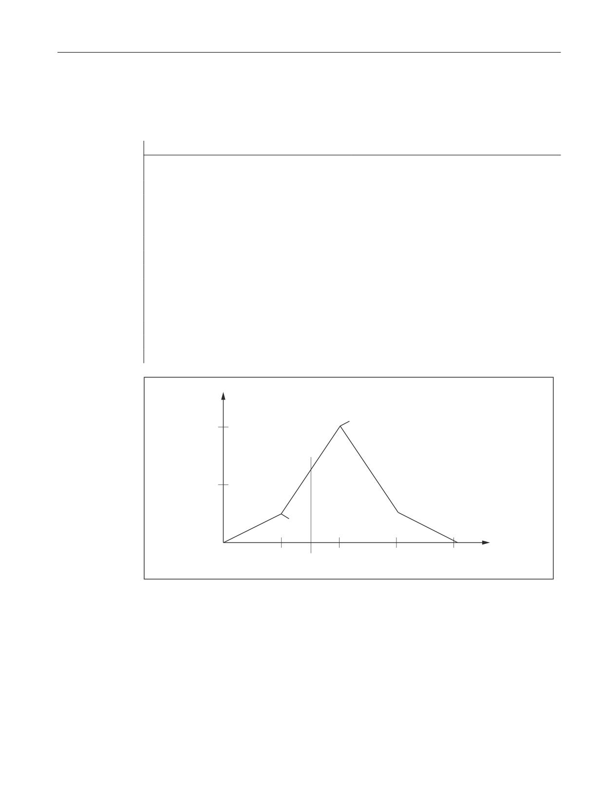
Identifying the segment associated with master value X
Example of reading the segment starting and end values for determining the curve segment
associated with master value X = 30 using CTABSSV and CTABSEV:
Program code
Comment
N10 DEF REAL STARTPOS
; Beginning of the definition for the
start position of the curve table
N20 DEF REAL ENDPOS
N30 DEF REAL GRADIENT
N100 CTABDEF(Y,X,1,0)
; Start of table definition
N110 X0 Y0
; Start position, 1st table segment
N120 X20 Y10
; End position, 1st table segment =
; Start position 2nd table segment
N130 X40 Y40
N140 X60 Y10
; 3. Curve segment
N150 X80 Y0
; 4. Curve segment
N160 CTABEND
; End of table definition
N200 STARTPOS=CTABSSV(30.0,1,GRADIENT)
; Start position Y in segment 2 = 10.
N210 ENDPOS=
; End position Y in segment 2 = 40
CTABSEV(30.0,1,GRADIENT)
; Segment 2 belongs to LW X = 30.0
<
(QG
1
1
1
1
6WDUW
;
;
Figure 10-2
Determining the curve segment associated with master value X = 30
Reading values at start and end
The values of the following axes and of the master axis at the start and end of a curve table
can be read with the following calls:
R10 =CTABTSV(n, degrees, F axis), following value at the beginning of the curve table
R10 =CTABTEV(n, degrees, F axis), following value at the beginning of the curve table
R10 =CTABTSP(n, degrees, F axis), following value at the beginning of the curve table
Special functions
Function Manual, 12/2018, A5E40874099B AB
421
M3: Coupled axes
10.2 Curve tables - 840D sl only
R10 =CTABTEP(n, degrees, F axis), following value at the beginning of the curve table
Value range of the following value
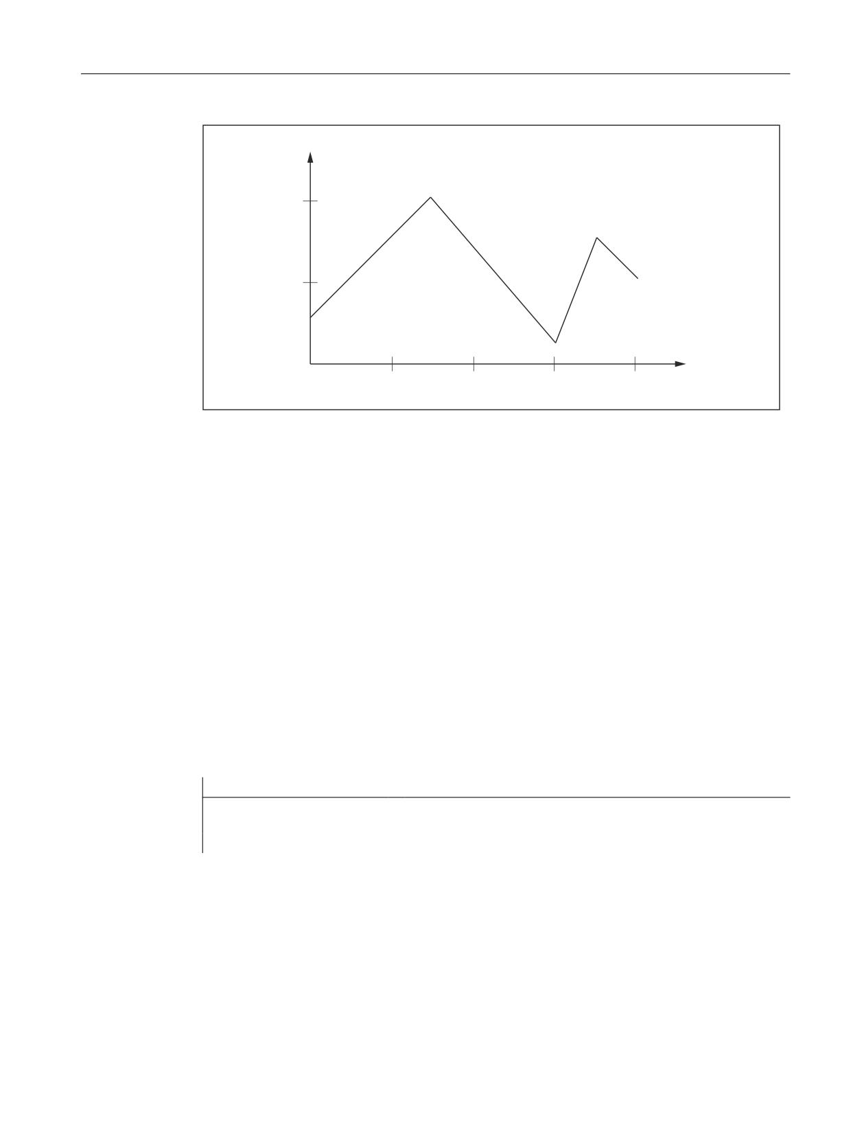
The following example illustrates how the minimum and maximum values of the table are
determined using CTABTMIN and CTABTMAX:
Program code
Comment
N10 DEF REAL STARTVAL
; Beginning of the definition for the start
and initial values of the curve table
N20 DEF REAL ENDVAL
N30 DEF REAL STARTPARA
N40 DEF REAL ENDPARA
N50 DEF REAL U_MINVAL
N60 DEF REAL U_MAXVAL
N70 DEF REAL GRADIENT
…
N100 CTABDEF(Y,X,1,0)
; Start of table definition
N110 X0 Y10
; Start value of the 1st table segment
N120 X30 Y40
; End position 1st table segment =
; start position 2nd table segment
N130 X60 Y5
; End position of the 2nd table segment ...
N140 X70 Y30
; End position of the 3rd curve segment ...
N150 X80 Y20
; End position of the 4th curve segment ...
N160 CTABEND
; End of table definition
N200 STARTPOS=CTABTSV(1,GRADIENT)
; STARTPOS = 10
; Start position of table as well as
N210 ENDPOS=CTABTEV(1,GRADIENT)
; ENDPOS = 20
; End position of table
N220 STARTPARA=CTABTSP(1,GRADIENT)
; STARTPARA = 0
; Master value at beginning of curve table
N230 ENDPARA=CTABTEP(1,GRADIENT)
; ENDPARA = 80
; Read master value at the end of the curve
table from the value range of the following
axis
N240 U_MINVAL=CTABTMIN(1)
; Minimum value when Y = 5 and
N250 U_MAXVAL=CTABTMAX(1)
; Maximum value when Y = 40
Special functions
422
Function Manual, 12/2018, A5E40874099B AB
M3: Coupled axes
10.2 Curve tables - 840D sl only
<
0D[LPXP
YDOXH
1
1
1
(QG
1
YDOXH
6WDUWLQJ
YDOXH
0LQLPXP
YDOXH
;
Figure 10-3
Determining the minimum and maximum values of the table
10.2.7
Activation/deactivation
Activation
The coupling of real axes to a curve table is activated through this command:
LEADON (<Following axis>, <Leading axis>, <n>)
with <n> =Number of the curve table
Activation is possible:
● In the part program
● in the definition of a synchronous action
Example:
N1000 LEADON(A,X,3)
; Axis A follows the master value X according to the rule
of motions defined in Curve Table No. 3
Deactivation
The switch off of the coupling to a curve table takes place through the following command:
LEADON (<Following axis>, <Leading axis>)
Special functions
Function Manual, 12/2018, A5E40874099B AB
423
M3: Coupled axes
10.2 Curve tables - 840D sl only
Deactivation is possible:
● In the part program
● in synchronized actions
Note
While programming LEADOF, the abbreviated form is also possible without specification of
the leading axis.
Example:
N1010 LEADOF(A,X)
; The coupling of Axis A with its leading axis is canceled
Multiple use
A curve table can be used several times in a single part program to couple different channel
axes.
10.2.8
Modulo-leading axis special case
Position is absolute
When an axial master value coupling is active, the position of the following axis via a curve
table is unique, i.e. an absolute assignment to the master axis exists.
This means that, when a modulo rotary axis is used as the master axis, the position of the
master axis is absolute. In other words, the position of the modulo rotary axis entered in the
curve table is absolute, and not modulo-reduced.
Example
Let the position of a modulo rotary axis with LEADON be 210°. The position 210° degrees is
used as the starting value in the curve table. After one rotation of the modulo axis, the axis
position is again displayed as 210°. The absolute position 570° is however taken as the input
value in the curve table:
210° + 1 round (360°) = 570°
10.2.9
Behavior in AUTOMATIC, MDA and JOG modes
Activation
An activated curve table is functional in the AUTOMATIC, MDA and JOG modes.
Special functions
424
Function Manual, 12/2018, A5E40874099B AB
M3: Coupled axes
10.2 Curve tables - 840D sl only
Basic setting after run-up
No curve tables are active after run-up.
10.2.10
Effectiveness of PLC interface signals
Dependent following axis
With respect to the motion of a following axis that is dependent on the leading axis, only the
following axis interface signals that effect termination of the motion (e.g. axis-specific feed
stop, axis inhibit, servo enable, etc.) are effective.
Leading axis
In an activated axis group, the interface signals move the leading axis through the axis coupling
to the associated following axis, i.e.:
● feed control of the leading axis causes a corresponding feed control of the following axis.
● A shutdown of the leading axis through interface signals (e.g., axis-specific feed stop, axis
inhibit, servo enable etc.) causes the corresponding following axis to shut down.
The effect of the axis inhibit of the leading axis on the following axis can be prevented through
the following MD setting:
MD37160 $MA_LEAD_FUNCTION_MASK, Bit 1 = 1
Position measuring system 1/2 (DB31, ... DBX1.5/1.6))
Switch-over of the position measuring system for the leading and following axes is not inhibited
for an active coupled axis group. The coupling is not canceled.
Recommendation: Switch the measuring system over when the coupling is deactivated.
10.2.11
Diagnosing and optimizing utilization of resources
The following functions allow parts programs to get information on the current utilization of
curve tables, table segments and polynomials.
One result of the diagnostic functions is that resources still available can be used
dynamically with the functions, without necessarily having to increase memory usage. The
description of the parameters in Chapter "Programming Curve Tables" also applies to the
following functions.
Special functions
Function Manual, 12/2018, A5E40874099B AB
425
M3: Coupled axes
10.2 Curve tables - 840D sl only
a) Curve tables
● Determine total number of defined tables.
The definition applies to all memory types (see also CTABNOMEM)
CTABNO()
● Number of defined tables in SRAM or DRAM of NC memory.
CTABNOMEM (memType)
If memType is not specified, the memory type specified in the following machine data:
MD20905 $MC_CTAB_DEFAULT_MEMORY_TYPE (default memory type for curve tables)
Result:
>= 0: Number of defined curve tables
-2: Invalid memory type
● Determine number of curve tables still possible in memory.
CTABFNO(memType)
If memType is not specified, the memory type specified in the following machine data:
MD220905 $MC_CTAB_DEFAULT_MEMORY_TYPE
Result:
>= 0: Number of possible tables
-2: Invalid memory type
● Determine the table number of the pth table in the memory type specified optionally
CTABID(p, memType)
If memType is not specified, the memory type specified in the following machine data:
MD20905 $MC_CTAB_DEFAULT_MEMORY_TYPE
Result:
Table number or
Alarm for invalid p or memType
When using the CTABID(p, memType) function, no assumptions should be made
regarding the sequence of the curve tables in the memory. The CTABID(p, ...) function
supplies the ID (table number) of the curve table entered in memory as the pth curve table.
If the sequence of curve tables in memory changes between consecutive calls of
CTABID()CTABID(), e.g. due to the deletion of curve tables with CTABDEL(), the
CTABID(p, ...) function can supply a different curve table with the same number.
Special functions
426
Function Manual, 12/2018, A5E40874099B AB
M3: Coupled axes
10.2 Curve tables - 840D sl only
To prevent this from happening, the curve tables concerned can be locked, using the
CTABLOCK(...) language command. In this case, it should be noted that the curve tables
concerned are then unlocked with CTABUNLOCK().
●
Determine block condition
Table n
CTABISLOCK(n)
Result:
> 0: Table is blocked
Reason for block:
1: by CTABLOCK()
2: by an active coupling
3: by CTABLOCK()and by an active coupling
= 0: Table is not blocked
- 1: Table does not exist
● Check whether the curve table exists
CTABEXISTS(n)
Result:
1: Table exists
0: Table does not exist
●
Determine memory type of a curve table
CTABMEMTYP(n)
Result:
0: Table in static SRAM NC memory
1: Table in dynamic "DRAM" NC memory
-1: Table does not exist
● by an active coupling periodic
CTABPERIOD(n)
Result:
0: Table is not periodic
1: Table is periodic in the leading axis
2: Table is periodic in the leading and following axes
-1: Table does not exist
b) Curve table segments
● Determine number of used curve segments of the type memType in the memory range.
● CTABSEG(memType, segType)
● If memType is not specified, the memory type specified in the following machine data:
MD20905 $MC_CTAB_DEFAULT_MEMORY_TYPE
Result:
>= 0: Number of curve segments
-2: Invalid memory type
If segType is not specified, the sum is produced via linear and polynomisl segments in the
memory type.
-2: segType not equal "L" or "P"
Special functions
Function Manual, 12/2018, A5E40874099B AB
427
M3: Coupled axes
10.2 Curve tables - 840D sl only
● Determine number of used curve segments of the type memType in the memory range
CTABSEGID(n, segType)
Result:
>= 0: Number of curve segments
-1: Curve table with number n does not exist
-2: segType not equal "L" or "P"
● Determine number of free curve segments of the type memType in the memory range
CTABFSEG(memType, segType)
If memType is not specified, the memory type specified in the following machine data:
MD20905 $MC_CTAB_DEFAULT_MEMORY_TYPE
Result:
>= 0: Number of free curve segments
-2: Invalid memory type, segType not equal "L" or "P"
● Determine maximum number of possible curve segments of the type segType in the memory
CTABMSEG(memType, segType)
If memType is not specified, the memory type specified in the following machine data:
MD20905 $MC_CTAB_DEFAULT_MEMORY_TYPE
Result:
>= 0: Maximum number of possible curve segments
-2: Invalid memory type, segType not equal "L" or "P"
c) Polynomials
● Determine the number of used polynomials of the memory type
CTABPOL(memType)
If memType is not specified, the memory type specified in the following machine data:
MD20905 $MC_CTAB_DEFAULT_MEMORY_TYPE
Result:
>= 0: Number of polynomials already used in the memory type
-2: Invalid memory type
● Determine the number of curve polynomials used by a curve table
CTABPOLID(n)
Result:
>=0: Number of used curve polynomials
-1: Curve table with number n does not exist
● Determine the number of free polynomials of the memory type
CTABFPOL(memType)
If memType is not specified, the memory type specified in the following machine data:
MD20905 $MC_CTAB_DEFAULT_MEMORY_TYPE
Result:
>= 0: Number of free curve polynomials
-2: Invalid memory type
● Determine the maximum number of polynomials of the memory type
CTABMPOL(memType)
If memType is not specified, the memory type specified in the following machine data:
MD20905 $MC_CTAB_DEFAULT_MEMORY_TYPE
Result:
>= 0: Maximum number of possible curve polynomials
-2: Invalid memory type
Special functions
428
Function Manual, 12/2018, A5E40874099B AB
M3: Coupled axes
10.2 Curve tables - 840D sl only
10.2.12
Supplementary conditions
Transformations
Transformations are not permissible in curve tables. TRAANG is an exception.
TRAANG
If TRAANG is programmed, the rule of motion programmed in the basic co-ordinate system is
transformed to the associated machine co-ordinate system. In this way it is possible to program
a curve table as Cartesian co-ordinates for a machine with inclined linear axes.
The condition that stipulates that "the direction of motion of the leading axis must not reverse
at any point of the rule of motion" must then be met in the machine co-ordinate system. Please
note that this condition in the basic co-ordinate system does not have the same meaning as
in the machine co-ordinate system, since the contour tangents are changed by the
transformation.
10.2.13
Examples
Definition of a curve table with linear sets
%_N_TAB_1_NOTPERI_MPF
;$PATH=/_N_WKS_DIR/_N_KURVENTABELLEN_WPD
; Def.TAB1 0-100mm Kue1/1 notperio.
N10 CTABDEF(YGEO,XGEO,1,0)
; FA=Y LA=X Curve No..=1 Not
period.
N1000 XGEO=0 YGEO=0
; Start values
N1010 XGEO=100 YGEO=100
CTABEND
M30
Definition of a curve table with polynomial sets
%_N_TAB_1_NOTPERI_MPF
;$PATH=/_N_WKS_DIR/_N_KURVENTABELLEN_WPD
; Def.TAB1 0-100mm Kue1/1 notperio.
N10 CTABDEF(Y,X,1,0)
; FA=Y LA=X Curve
No..=1 Not period.
N16 G1 X0.000 Y0.000
N17 POLY PO[X]=(31.734,0.352,-0.412) PO[Y]=(3.200,2.383,0.401)
N18 PO[X]=(49.711,-0.297,0.169) PO[Y]=(7.457,1.202,-0.643)
N19 PO[X]=(105.941,1.961,-0.938) PO[Y]=(11.708,-6.820,-1.718)
N20 PO[X]=(132.644,-0.196,-0.053) PO[Y]=(6.815,-2.743,0.724)
Special functions
Function Manual, 12/2018, A5E40874099B AB
429

M3: Coupled axes
10.2 Curve tables - 840D sl only
%_N_TAB_1_NOTPERI_MPF
N21 PO[X]=(147.754,-0.116,0.103) PO[Y]=(3.359,-0.188,0.277)
N22 PO[X]=(174.441,0.578,-0.206) PO[Y]=(0.123,1.925,0.188)
N23 PO[X]=(185.598,-0.007,0.005) PO[Y]=(-0.123,0.430,-0.287)
N24 PO[X]=(212.285,0.040,-0.206) PO[Y]=(-3.362,-2.491,0.190)
N25 PO[X]=(227.395,-0.193,0.103) PO[Y]=(-6.818,-0.641,0.276)
N26 PO[X]=(254.098,0.355,-0.053) PO[Y]=(-11.710,0.573,0.723)
N26 PO[X]=(254.098,0.355,-0.053) PO[Y]=(-11.710,0.573,0.723)
N27 PO[X]=(310.324,0.852,-0.937) PO[Y]=(-7.454,11.975,-1.720)
N28 PO[X]=(328.299,-0.209,0.169) PO[Y]=(-3.197,0.726,-0.643)
N29 PO[X]=(360.031,0.885,-0.413) PO[Y]=(0.000,-3.588,0.403)
CTABEND
N30 M30
Definition of a periodic curve table
Table No: 2
Master value range: 0 - 360
The following axis traverses from N70 to N90, a movement from 0 to 45 and back to 0.
N10 DEF REAL DEPPOS
N20 DEF REAL GRADIENT
N30 CTABDEF(Y,X,2,1)
N40 G1 X=0 Y=0
N50 POLY
N60 PO[X]=(45.0)
N70 PO[X]=(90.0) PO[Y]=(45.0,135.0,-90)
N80 PO[X]=(270.0)
N90 PO[X]=(315.0) PO[Y]=(0.0,-135.0,90)
N100 PO[X]=(360.0)
N110 CTABEND
N130 G1 F1000 X0
; Testing the curve by coupling Y to X
N140 LEADON(Y,X,2)
N150 X360
N160 X0
N170 LEADOF(Y,X)
N180 DEPPOS = CTAB(75.0,2,GRADIENT)
; Reading the table position at master
value 75.0 from the curve table with
Table No. 2
N190 G0 X75 Y=DEPPOS
; Positions of leading and following
axis
N200 LEADON(Y,X,2)
; No synchronization of the following
axis is required after the coupling
is activated
N210 G1 X110 F1000
N220 LEADOF(Y,X)
Special functions
430
Function Manual, 12/2018, A5E40874099B AB
M3: Coupled axes
10.3 Master value coupling - 840D sl only
N10 DEF REAL DEPPOS
N230 M30
10.3
Master value coupling - 840D sl only
10.3.1
Product brief
10.3.1.1
Function
The "axial master value coupling" function can be used to process short programs cyclically
with close coupling of the axes to one another and a master value that is either generated
internally or input from an external source.
The master value can, for example, be derived from a conveyor belt or a vertical shaft.
The axial master value coupling can be switched on and off in the NC part program or via
synchronized action.
10.3.1.2
Preconditions
The option "Master Value Coupling and Curve Tables Interpolation" or the relevant option of
generic coupling (refer to " Preconditions (Page 470) " in the "Brief description" for generic
coupling) is a prerequisite for utilization of the function.
10.3.2
General functionality
Curve table
With the axial master value coupling, a leading and a following axis are moved in synchronism.
It is possible to assign the position of the following axis via a curve table or the resulting
polynomial uniquely to a position of the leading axis - simulated if necessary.
Master value object
The master value object is the input variable for the curve table.
The following can be defined as the position of the master value object:
● The axis actual position (actual value measured by transmitter)
or
● The setpoint position (calculated from interpolator) (default)
If the leading axis is interpolated by the same NCU, the setpoint coupling delivers a better
follow-up response than is possible for actual value coupling (in the same IPO cycle).
Special functions
Function Manual, 12/2018, A5E40874099B AB
431
M3: Coupled axes
10.3 Master value coupling - 840D sl only
Virtual leading axis / simulated master value
If the leading axis is not interpolated by the same NCU, the interpolator that is implemented
in the NCU for this particular leading axis can be used for master value simulation. The following
machine data settings must be defined for this:
MD30132 $MA_IS_VIRTUAL_AX[n] = 1 (axis is virtual axis)
MD30130 $MA_CTRLOUT_TYPE[n] = 0 (simulation as output type of setpoint)
Properties of master value simulation:
● Separation of IPO and servo.
● Actual values of the axis are recorded.
● Setpoint values are produced by IPO but not passed on to the servo motor.
● When switching over to master value coupling, the simulation can be programmed with the
last actual value read, whereas the path of the actual value is generally outside the control
of the NCU.
● If, for purposes of master value simulation, the master value object is switched from actual
value coupling to setpoint value coupling and a traversing command is issued for the leading
axis in the same interpolator clock cycle, the interpolator for the axis is initialized by the NC
so that the master value produces a constant path in the first derivation.
Note
Virtual axes assigned to a real drive must remain unblocked.
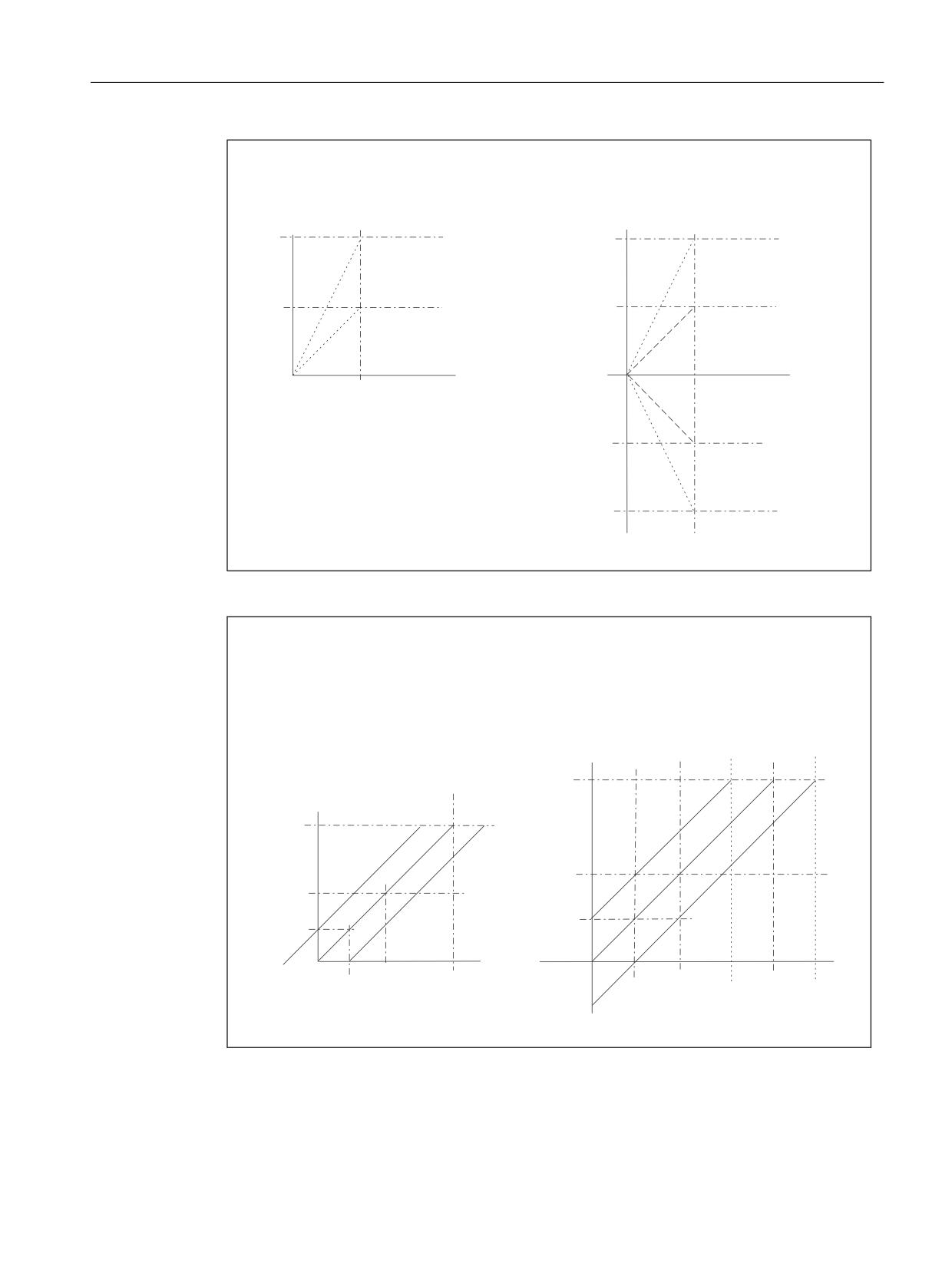
Offset and scaling
The setpoint value for the following axis can be offset and scaled. The following setting data
is used for this:
SD43102 $SA_LEAD_OFFSET_IN_POS (offset of master value with coupling to this axis)
SD43104 $SA_LEAD_SCALE_IN_POS (scaling of master value with coupling to this axis)
SD43106 $SA_LEAD_OFFSET_OUT_POS (offset of function value of the curve table)
SD43108 $SA_LEAD_SCALE_OUT_POS (scaling of function value of the curve table)
If (x) is a periodic curve table and this is interpreted as oscillation, the offset and scaling can
also be interpreted as follows:
SD43102 $SA_LEAD_OFFSET_IN_POS[Y] offsets the phase of the oscillation.
SD43106 $SA_LEAD_SCALE_OUT_POS[Y] affects the amplitude.
SD43108 $SA_LEAD_OFFSET_OUT_POS[Y] offsets the center of the oscillation
If the coupling is activated and synchronous, the new set position is approached as soon as
values are written to this setting data.
Special functions
432
Function Manual, 12/2018, A5E40874099B AB
M3: Coupled axes
10.3 Master value coupling - 840D sl only
6'
6$B/($'B6&$/(B,1B326>)$@
6'
6$B/($'B6&$/(B287B326>)$@
7KH LQSXW YDOXH LV PXOWLSOLHG
7KH RXWSXW YDOXH LV PXOWLSOLHG 6HWWLQJ GDWD LV
HIIHFWLYH RXWVLGH RI WKH WDEOH GHILQLWLRQ DOVR LQ
WKH QHJDWLYH GLUHFWLRQ
)$
PP
PP
)$
PP
PP
/$
/$
PP
PP
PP
PP
PP
PP
7DEOH GHILQLWLRQ IRU H[DPSOH
PP
&7$%'() )$ /$ &7$%15
/$
)$
/$
)$
&7$%(1'
PP
:LWK ,1 6&$/( LV QRW DFWLYH
RXWVLGH 7$%
:LWK 287 6&$/( LV DFWLYH RXWVLGH 7$%
Figure 10-4
Master value coupling offset and scaling (multiplied)
6'
B 6$B/($'B2))6(7B,1B326>)$@
6'
6$B/($'B2))6(7B287B326>)$@
7KH FDOFXODWHG SRVLWLRQ RI WKH IROORZLQJ D[LV LV
7KH FDOFXODWHG SRVLWLRQ RI WKH IROORZLQJ D[LV LV
RIIVHW ZLWK WKH VSHFLILHG LQFUHPHQWV
RIIVHW ZLWK WKH VSHFLILHG LQFUHPHQWV ,I WKH 7$% LV
PRYHG RXWVLGH RI WKH )$ /($'21 SRVLWLRQ .23
FDQQRW EH VZLWFKHG RQ 6HWWLQJ GDWD LV HIIHFWLYH
RXWVLGH RI WKH WDEOH GHILQLWLRQ DOVR LQ WKH
QHJDWLYH GLUHFWLRQ
)$
PP
PP
PP
)$
PP
PP
PP
PP
QHZ /$
ZLWK ಱ
ಯ
/$
/$
PP
PP
PP
PP
PP
PP
PP
PP
:LWK ,1 2))6(7 LV QRW DFWLYH RXWVLGH 7$%
:LWK 287 2))6(7 DFWLYH RXWVLGH 7$%
Figure 10-5
Master value coupling offset and scaling (with increment offset)
Special functions
Function Manual, 12/2018, A5E40874099B AB
433
M3: Coupled axes
10.3 Master value coupling - 840D sl only
Reaction to Stop
All leading value coupled following axes react to channel stop and MODE GROUP stop.
Master value coupled following axes react to a stop due to end of program (M30, M02) if they
have not been activated by static synchronized actions (IDS=...). The following machine
data is to be observed in this connection:
MD20110 $MC_RESET_MODE_MASK (definition of initial control settings after RESET / TP
End)
MD20112 $MC_START_MODE_MASK (definition of initial control settings for NC-START)
Leading axis and following axis must always interpolate in the same channel. A following axis
located in a different channel cannot be coupled (axis replacement).
START and mode change enable a following axis in the master value coupling that has been
stopped.
RESET also enables a stopped following axis in master value coupling. If enabling by RESET
is not desired, or if it is dangerous (e.g. because the following axis is coupled to an external
master value not controlled by the NC), then MD20110 must be programmed such that master
value couplings are switched off with RESET (=2001H, i.e. bit 13 set to 1).
Axial functions
Actual value coupling causes a position offset between the leading and following axis. The
cause of this is the IPO cycle-based dead time in the position controller, which lies between
the actual value of the leading axis and the following axis.
Normally, the position offset and the following error is compensated by a linear extrapolation
of the master value to the extent of this dead time, i.e. dead time compensation is active in
master value coupling. The following MD setting is defined to deactivate the dead time
compensation:
MD37160 $MA_LEAD_FUNCTION_MASK Bit 0 = 0
Interface to axis exchange
A master value coupled following axis receives its setpoint values from curve tables. Overlaid
programming of this axis is not possible in the part program. Therefore, the master value-
coupled following axis is removed from the channel in the same way as for axis exchange.
This is carried out automatically when the coupling is activated in the part program.
If the coupling is to be activated with synchronized action, then it must be prepared for it in
advance with RELEASE.
After a master value coupling has been deactivated, the former following axis can be
programmed again in the part program.
Spindles in master value coupling
A spindle can only be used as the master value coupled following axis if it has been switched
to axis mode beforehand. The machine data parameter block of the axis drive then applies.
Special functions
434
Function Manual, 12/2018, A5E40874099B AB
M3: Coupled axes
10.3 Master value coupling - 840D sl only
Example: Activation from synchronized action
Program code
Comment
SPOS=0
B=IC(0)
; switch spindle to axis operation.
RELEASE(Y)
; Enable for synchronized action.
ID=1 WHEN ($AA_IM[X]<-50) DO LEADON(B,X,2)
; Y is coupled to X via curve table No.
2.
10.3.3
Programming
Definition and activation
An axis master value coupling is defined and activated simultaneously with the modal effective
language command LEADON.
Syntax:
LEADON(<FA>,<LA>,<CTABn>)
Meaning:
<FA>
Following axis as geometry-, channel- or machine axis name (X, Y, Z,...)
<LA>
Leading axis as geometry-, channel- or machine axis name (X, Y, Z,...)
Software axis is also possible:
MD30130 $MA_CTRLOUT_TYPE=0 (setpoint output type)
<CTABn>
Number of curve table
Range of values:
1 to 999
Example:
Program code
Comment
LEADON(Y,X,1)
; Definition and activation of a master value coupling between
the leading axis X and the following axis Y. Curve Table No.
1 should be used to calculate the following value.
Special functions
Function Manual, 12/2018, A5E40874099B AB
435
M3: Coupled axes
10.3 Master value coupling - 840D sl only
Boundary conditions:
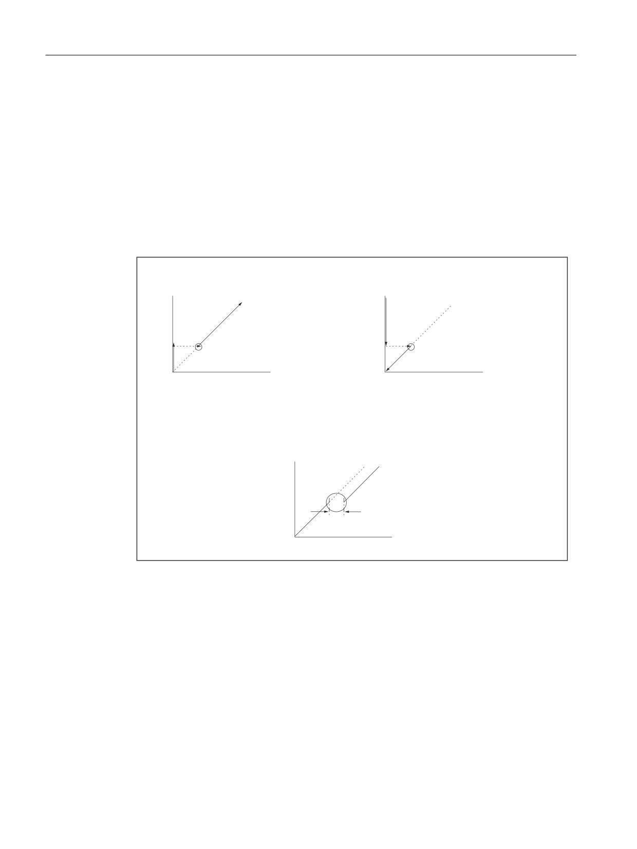
● No reference point is required to activate the coupling.
● A defined following axis cannot be traversed in the JOG mode (not even if the "Synchronized
run fine" or. "synchronized run coarse" interface signal is not there).
● An activated coupling must first be deactivated with LEADOF before it can be activated again
with LEADON. The settings in the following machine data are to be considered in this
connection:
MD20112 MC_START_MODE_MASK (definition of initial control system settings with NC-
START)
MD20110 $MC_RESET_MODE_MASK (definition of initial control settings after RESET/TP-
End)
&283/,1* 21 DQG V\QFKURQRXV ZLWK )$ SRVLWLRQ
/HDGLQJ D[LV
/HDGLQJ D[LV
7UDYHUVLQJ GLUHFWLRQ
7UDYHUVLQJ GLUHFWLRQ
&283/,1* 21
&283/,1* 21
)ROORZLQJ D[LV
)ROORZLQJ D[LV
.23 LV RQO\ VZLWFKHG RQ ZKHQ WKH /$ LV
.23 LV RQO\ VZLWFKHG RQ ZKHQ WKH /$ LV
ZLWKLQ WKH WDEOH UDQJH RI WKH )$
ZLWKLQ WKH WDEOH UDQJH RI WKH )$
2YHUOD\LQJ DIWHU &283/,1* 21 ZLWK KDQGZKHHO '5)
/HDGLQJ D[LV
,Q WKH FRXSOHG VWDWH WKH IROORZLQJ D[LV FDQ EH
RYHUODLG ZLWK %$ $872 '5)
2YHUULGH
)ROORZLQJ D[LV
Figure 10-6
Activating master value coupling
Switch off
An axis master value coupling is deactivated with the model language command LEADOF.
When the axis master value coupling is deactivated, the following axis becomes the command
axis and a stop command is generated implicitly for the following axis. The stop command can
be overwritten by another command with a synchronous action.
Syntax:
LEADON(<FA>,<LA>)
Special functions
436
Function Manual, 12/2018, A5E40874099B AB

M3: Coupled axes
10.3 Master value coupling - 840D sl only
Meaning:
<FA>
Following axis as geometry-, channel- or machine axis name (X, Y, Z,...)
<LA>
Leading axis as geometry-, channel- or machine axis name (X, Y, Z,...)
Software axis is also possible:
MD30130 $MA_CTRLOUT_TYPE=0 (setpoint output type)
Example:
Program code
Comment
LEADOF(Y,X,1)
; Switching off of master value coupling between the leading
axis X and the following axis Y.
Note
Activating / deactivating the axis master value coupling with LEADON / LEADOF is permissible
both in the part program and in synchronous actions.
References:
Function Manual, Synchronized Actions
Coupling type
The coupling type is defined by the following axis-specific setting data:
SD43100 $SA_LEAD_TYPE[<LA>] (type of master value)
<LA>: Leading axis as geometry axis name, channel axis name or machine axis name (X, Y,
Z,...)
Value
Meaning
0
Actual value coupling (this type of coupling must be used for external leading axes)
1
Setpoint coupling (default setting)
2
Simulated master value (note virtual axis, not evaluated for FA)
Switch-over between actual and setpoint value coupling is possible at any time (preferably in
the idle phase).
Special functions
Function Manual, 12/2018, A5E40874099B AB
437
M3: Coupled axes
10.3 Master value coupling - 840D sl only
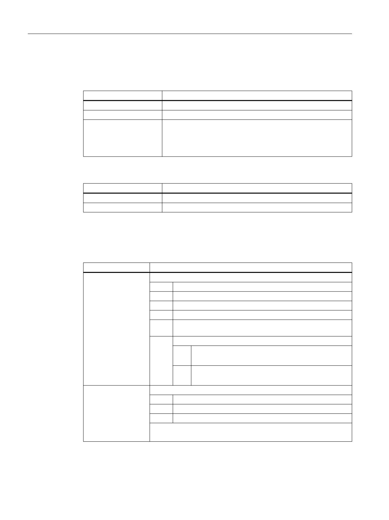
System variables of the master value
The following master value system variables can only be read from part program and from
synchronous actions:
System variable
Meaning
$AA_LEAD_V[ax]
Velocity of the leading axis
$AA_LEAD_P[ax]
Position of the leading axis
$AA_LEAD_P_TURN
Master value position
Portion that is deducted during modulo reaction.
The actual (not modulo-reduced) position of the leading axis is:
$AA_LEAD_P_TURN + $AA_LEAD_P
The speeds and positions of simulated master values (when $SA_LEAD_TYPE[ax]=2) can be
written in and read from the part program and synchronous actions.
System variable
Meaning
$AA_LEAD_SV[ax]
Simulated master value velocity per IPO cycle
$AA_LEAD_SP[ax]
Simulated position in MCS
System variables of the following axis
For the following axis, the following system variables can be read in the part program and
synchronized action:
System variable
Meaning
$AA_SYNC[ax]
Condition of the coupling between following and leading axes
Value
Meaning
0
not synchronized
1
"Coarse synchronous operation" 1)
2
"Fine synchronous operation" 2)
3
"Coarse synchronous operation" 1) AND "Fine synchronous opera-
2)
tion"
Corresponds to:
1)
● MD37200 $MA_COUPLE_POS_TOL_COARSE
● DB31, ... DBX98.1 (coarse synchronous operation)
2)
● MD37210 $MA_COUPLE_POS_TOL_FINE
● DB31, ... DBX98.0 (fine synchronous operation)
$AA_IN_SYNC[ax]
Condition of the synchronization between following and leading axes
Value
Meaning
0
Synchronization not started or ended.
1
Synchronization is running, i. e., the following axis is synchronized.
$AA_IN_SYNC[ax] corresponds to the NC/PLC interface signal:
DB31, ... DBX99.4 (synchronization running)
Special functions
438
Function Manual, 12/2018, A5E40874099B AB
M3: Coupled axes
10.3 Master value coupling - 840D sl only
Note
If the following axis is not enabled for travel, it is stopped and is no longer synchronous.
10.3.4
Behavior in AUTOMATIC, MDA and JOG modes
Efficiency
A master value coupling is active depending on the settings in the part program and in the
following machine data:
MD20110 $MC_RESET_MODE_MASK (definition of initial control settings after RESET / TP
End)
MD20112 $MC_START_MODE_MASK (definition of initial control system settings with NC-
START)
Manual mode
Once a master axis coupling has been activated, traversal of the master axis (e.g. with rapid
traverse or incremental dimension INC1 ... INC10000) results in a movement of the slave axis,
allowing for the curve table definition.
Referencing
A master value coupled-following axis should be referenced prior to activation of the coupling.
A following axis cannot be referenced when the coupling is activated.
Deletion of distance-to-go
When deletion of distance-to-go is performed for a leading axis, all axes in the associated,
activated master value coupling are shut down.
Basic setting after POWER ON
No master value couplings are active after POWER ON. (Options with ASUB).
Behavior after NC start/RESET
The following behavior results, depending on the settings of the machine data:
MD20110 $MC_RESET_MODE_MASK (bit 13) (definition of initial control settings after
RESET / TP End)
Special functions
Function Manual, 12/2018, A5E40874099B AB
439
M3: Coupled axes
10.3 Master value coupling - 840D sl only
MD20112 $MC_START_MODE_MASK (bit 13) (definition of initial control system settings with
NC-START)
● MD20110 $MC_RESET_MODE_MASK=2001H
&&
MD20112 $MC_START_MODE_MASK=0H
→ Master value coupling remains valid after RESET and START
● MD20110 $MC_RESET_MODE_MASK=2001H
&&
MD20112 $MC_START_MODE_MASK=2000H
→ Master value coupling remains valid after RESET and is canceled with START. However,
master value coupling activated via IDS=... remains valid.
● MD20110 $MC_RESET_MODE_MASK=1H
→ Master value coupling is canceled with RESET irrespective of machine data:
MD20112 $MC_START_MODE_MASK
Master value coupling activated via IDS=... can only be deactivated via an operator front
panel reset and remains valid after program end/reset (M30, M02).
● MD20110 $MC_RESET_MODE_MASK=0H
→ Master value coupling remains valid after RESET and is canceled with START, irrespective
of machine data:
MD20112 $MC_START_MODE_MASK
However, master value coupling activated via IDS=... remains valid.
Reference:
Function Manual, Basic Functions; Coordinate Systems, Axis Types,
Axis Configurations, ... (K2)
Activating, deactivating
Master value couplings activated via a static synchronous action (IDS=...) are:
● not deactivated during program start, regardless of the value of machine data:
MD20110 $MC_RESET_MODE_MASK (definition of initial control settings after RESET /
TP End)
and
MD20112 $MC_START_MODE_MASK (definition of initial control system settings with NC-
START)
● not deactivated during program end reset (M30, M02), regardless of the value of machine
data:
MD20110 $MC_RESET_MODE_MASK
Special functions
440
Function Manual, 12/2018, A5E40874099B AB
M3: Coupled axes
10.3 Master value coupling - 840D sl only
10.3.5
Effectiveness of PLC interface signals
Leading axis
When a coupled axis group is active, the interface signals (IS) of the leading axis are applied
to the appropriate following axis via axis coupling. i.e.:
● a feed control action of the leading axis is applied via the master value coupling to effect
an appropriate feed control action in the following axis.
● shutdown of the leading axis as the result of an IS (e.g. axis-specific feed stop, axis inhibit,
servo enable, etc.) causes the corresponding coupled motion axis to shut down.
Position measuring system 1/2 (DB31, ... DBX1.5/1.6))
Switch-over of the position measuring system for the leading and following axes is not inhibited
for an active coupled axis group. The coupling is not canceled.
Recommendation: Switch the measuring system over when the coupling is deactivated.
10.3.6
Special characteristics of the axis master value coupling function
Control dynamics
Depending on the application in question, it may be advisable to match the position controller
parameter settings (e.g. servo gain factor (KVfactor)) of the leading axis and following axis in
an axis grouping. It may be necessary to activate other parameter sets for the following axis.
The dynamics of the following axis should be the same or better than those of the leading axis.
Status of coupling
See Chapter "Status of coupling (Page 404)"
Actual value display
The display of the actual value is updated for all axes of in a master value coupled axis grouping
(only real axes) coupled via a master value.
Interpolation
When the movement defined in the curve table is interpolated, axis position and axis speed
are calculated for a master value and its speed.
Logging
The curve tables generated by the definition of motion sequences are stored in the battery-
backed memory.
Special functions
Function Manual, 12/2018, A5E40874099B AB
441
M3: Coupled axes
10.4 Electronic gear (EG)
The curve tables are not lost when the control system is switched off.
These functions have no effect on cyclic machines because they are performed without
operator actions. Nor does it make sense to perform automatic (re-)positioning via the NC with
external master values.
10.3.7
Supplementary conditions
External master value axes
When using the REPOS or REPOSA parts program instructions in conjunction with external
master value axes, it should be ensured that these are released by the channel or switched
to a "neutral state" using the RELEASE instruction.
When attempting to reposition without release of the axis, the message "Wait: Feed stop active"
is displayed and the processing of the part program is not continued.
10.4
Electronic gear (EG)
10.4.1
Product brief
10.4.1.1
Function
General
The "electronic gear" function makes it possible to control the movement of a following axis,
depending on up to five master axes. The relationship between each leading axis and the
following axis is defined by the coupling factor. Following axis motion components derived
from the individual leading axis motion components have an additive effect.
The coupling can be based on:
● Actual value of the leading axis
● Setpoint of the leading axis
The following functions of a gear grouping can be programmed using part program instructions:
● Defining
● Switch on
● Switch off
● Delete
Special functions
442
Function Manual, 12/2018, A5E40874099B AB
M3: Coupled axes
10.4 Electronic gear (EG)
Curve tables
Non-linear relationships between lead and following axes can also be implemented using curve
tables.
Cascading
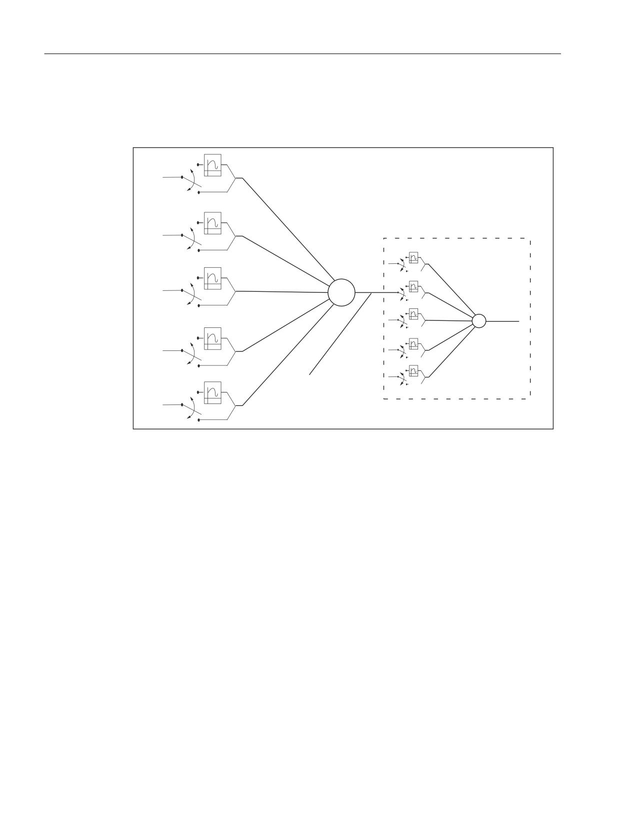
Electronic gearboxes can be cascaded, i.e. the following axis of an electronic gearbox can be
the leading axis for a subsequent electronic gearbox.
Synchronous position
An additional function for synchronizing the following axis allows a synchronous position to be
selected:
● Approach next division (tooth gap) time-optimized
● Approach next division (tooth gap) path-optimized
● Approach in positive direction of axis rotation, absolute
● Approach in negative direction of axis rotation, absolute
● Traverse time-optimized with respect to programmed synchronized position
● Traverse path-optimized with respect to programmed synchronized position
Application Examples:
● Machine tools for gear cutting
● Gear trains for production machines
10.4.1.2
Preconditions
The "Electronic Gearbox" option or the relevant option of generic coupling (refer to
" Preconditions (Page 470) " in the "Brief description" of Generic Coupling) is required for the
usage of function.
10.4.2
Electronic gear (EG)
Function
With the aid of the "Electronic gearbox" the movement of a following axis FA can be interpolated
dependent of up to five leading axes LA. The relationship between each leading axis and the
following axis is defined by a coupling factor. The following axis motion components derived
in this manner from the individual leading axis motion components have an additive effect.
FAset = SynPosFA + (LA1-SynPosLA1)*CF1 +... +(LA5-SynPosLA5)*CF5
with:
SynPosFA, SynPosLAi: from call EGONSYN (see below)
FAsetpoint: Partial setpoint of the following axis.
Special functions
Function Manual, 12/2018, A5E40874099B AB
443
M3: Coupled axes
10.4 Electronic gear (EG)
LA
i
: Setpoint or actual value of the ith leading axis (depending on the type of coupling - see
below)
KFi: Coupling factor of the ith leading axis (see below)
All paths are referred to the basic co-ordinate system BCS.
When an EG axis group is activated, it is possible to synchronize the leading axes and following
axis in relation to a defined starting position.
From the part program a gearbox group can be:
● defined,
● activated,
● deactivated,
● deleted.
Extensions
The influence of each of the 5 leading axes can be specified using a curve table as an
alternative to a transmission ratio (KF=numerator/denominator).
It is thus possible for each curve (except for the special case of a straight line) for the leading
axis to influence the following axis in a non-linear manner. The function can only be used with
EGONSYN.
The function EG can be activated with curve tables with EGON.
The function EGONSYNE is available for approaching the synchronized position of the
following axis with a specified approach mode.
For special applications, it may be advisable configure the position controller as a PI
controller.
CAUTION
Application faults
Knowledge of the control technology and measurements with servo trace are an absolute
prerequisite for using this function.
References:
● CNC Commissioning Manual: NC, PLC, Drive
● Function Manual, Basic Functions; Velocities, Setpoint-Actual Value Systems, Closed-
Loop Control (G2)
Coupling type
The following axis motion can be derived from either of the following:
● Setpoints of leading axes
● Actual values of leading axes
The reference is set in the definition call for the EG axis group:
Special functions
444
Function Manual, 12/2018, A5E40874099B AB
M3: Coupled axes
10.4 Electronic gear (EG)
EGDEF
(see Chapter "Definition of an EG axis group (Page 451)")
Coupling factor
The coupling factor must be programmed for each leading axis in the group. It is defined by
numerator/denominator.
Coupling factor values numerator and denominator are entered per leading axis with the
following activation calls:
EGON
EGONSYN
EGONSYNE
(see Chapter "Activating an EG axis group (Page 452)")
Number of EG axis groups
Several EG axis groups can be defined at the same time. The maximum possible number of
EG axis groupings is set in the following machine data:
MD11660 $MN_NUM_EG
The maximum permissible number of EG axis groups is 31.
Note
The option must be enabled.
Special functions
Function Manual, 12/2018, A5E40874099B AB
445
M3: Coupled axes
10.4 Electronic gear (EG)
EG cascading
The following axis of an EG can be the leading axis of another EG. For a sample configuration
file, see Chapter "Examples".
/$
=
1
/$
&DVFDGLQJ DOVR SRVVLEOH
=
1
/$.
=1
/$
/$.
=
=1
1
/$.
=1
/$.
/$
=1
=
/$.
1
ಯ6RIWZDUHರ D[LV
=1
/$
=
1
Figure 10-7
Block diagram of an electronic gearbox
Synchronous positions
To start up the EG axis group, an approach to defined positions for the following axis can first
be requested.
Synchronous positions are specified with:
EGONSYN (see below for details)
EGONSYNE (extended EGONSYN call).
Synchronization
If a gear is started with EGON(), EGONSYN() or EGONSYNE() see below, the actual position
of the following axis is only identical to the setpoint position defined by the rule of motion of
the gear specified by the positions of the leading axes at this time if the part program developer
makes sure that it is. The control then uses the motion of the following axis to ensure that the
setpoint and actual positions of the following axes correspond as quickly as possible if the
leading axes are moved further. This procedure is called synchronization. After synchronization
of the following axis, the term synchronous gearing is used.
Special functions
446
Function Manual, 12/2018, A5E40874099B AB
M3: Coupled axes
10.4 Electronic gear (EG)
Activation response
An electronic gearbox can be activated in two different ways:
1. On the basis of the axis positions that have been reached up to now in the course of
processing the command to activate the EG axis group is issued without specifying the
synchronizing positions for each individual axis.
EGON (see Chapter "Activating an EG axis group (Page 452)")
2. The command to activate the EG axis group specifies the synchronized positions for each
axis. From the point in time when these positions are reached, the EG should be
synchronized.
EGONSYN (see Chapter "Activating an EG axis group (Page 452)")
3. The command to activate the EG axis group specifies the synchronized positions and
approach mode for each axis. From the point in time when these positions are reached,
the EG should be synchronized.
EGONSYNE (see Chapter "Activating an EG axis group (Page 452)")
Synchronization with EGON
With EGON(), no specifications are made for the positions at which the following axis is to be
synchronized. The control system activates the EG and issues the signal "Synchronized
position reached".
Synchronization for EGONSYN
1. With EGONSYN(), the positions of the leading axes and the synchronization position for
the following axis are specified by the command.
● The control then traverses the following axis with just the right acceleration and velocity to
the specified synchronization position so that the following axis is in position with the leading
axes at its synchronization position.
● If the following axis is stationary: If the "Feed stop/spindle stop" DB 31, ... DBX 4.3 is set
for the following axis, the following axis is not set in motion by EGON or EGONSYN. A
traverse command is issued and block changing is blocked until the axis-specific feed is
enabled. EGOSYN is topped by RESET transformed into EGON. The programmed
synchronized positions are deleted.
● If the following axis is not stationary: The NST "Feed Stop/Spindle Stop" DB31, ... DBX4.3
has no direct influence on the electronic gearbox. As before, it does have an indirect effect
on the leading axes, if these are located in the same channel.
● For channel specific feed enabling and for override nothing is implemented. Override still
has no direct influence on the electronic gearbox. The axis-specific feed enable is set,
depending on the current override setting.
Synchronization for EGONSYNE
With EGONSYN(), the positions of the leading axes and the synchronization position for the
following axis are specified by the command.
The control system moves the following axis to the synchronized position according to the
program approach mode.
Special functions
Function Manual, 12/2018, A5E40874099B AB
447
M3: Coupled axes
10.4 Electronic gear (EG)
Synchronization abort with EGONSYN and EGONSYNE
1. The EGONSYN/EGONSYNE command is aborted under the following conditions and
changed to an EGON command:
● RESET
● Axis switches to tracking
The defined synchronization positions are ignored. Synchronous traverse monitoring still takes
synchronized positions into account.
Aborting position synchronization generates alarm 16774.
The alarm may be suppressed with the following machine data:
MD11410 $MN_SUPPRESS_ALARM_MASK Bit31 = 1
Synchronous monitoring
The synchronism of the gearbox is monitored in each interpolator clock cycle on the basis of
the actual values of the following and leading axes. For this purpose, the actual values of the
axes are computed according to the rule of motion of the coupling. The synchronism
difference is the difference between the actual value of the following axis and the value
calculated from the leading axis actual values according to the rule of motion. The synchronism
difference can be queried from the part program (see below).
Changes in the synchronism difference
The mass inertia of the axis systems during acceleration can cause dynamic fluctuations in
the synchronism difference. The synchronism difference is checked continuously and the
tolerance values in the machine data used to produce interface signals.
The synchronism difference is compared with the following machine data:
MD37200 $MA_COUPLE_POS_TOL_COARSE
MD37210 $MA_COUPLE_POS_TOL_FINE
Depending on the result of this comparison, the following signals are set:
NST "Synchronous travel fine" DB31, ... DBX98.0
NST "synchronous traverse coarse" DB31, ... DBX98.1
Difference > .. TOL_COARSE
As long as the synchronism difference is greater than the following machine data, the gearbox
is not synchronized and neither IS "Coarse synchronism" DB 31, ... DBX 98.1 nor IS "Fine
synchronism" DB 31, ... DBX 98.0 is active:
MD37200 $MN_COUPLE_POS_TOL_COARSE
Instead, the following interface signal is displayed:
NST "synchronization running" DB31, ... DBX99.4
Special functions
448
Function Manual, 12/2018, A5E40874099B AB
M3: Coupled axes
10.4 Electronic gear (EG)
Difference < .. TOL_COARSE
As long as the synchronism difference is smaller than the following machine data, IS "Coarse
synchronism" DB 31, ... DBX 98.1 is at the interface and IS "Fine synchronism" DB31, ...
DBX99.4 is deleted:
MD37200 $MN_COUPLE_POS_TOL_COARSE
Difference > .. TOL_FINE
If the synchronism difference is smaller than the following machine data, then NST
"synchronous traverse fine" DB31, ... DBX98.0 is at the interface:
MD37210 $MA COUPLE_POS_TOL_FINE
Synchronism difference for EG cascades
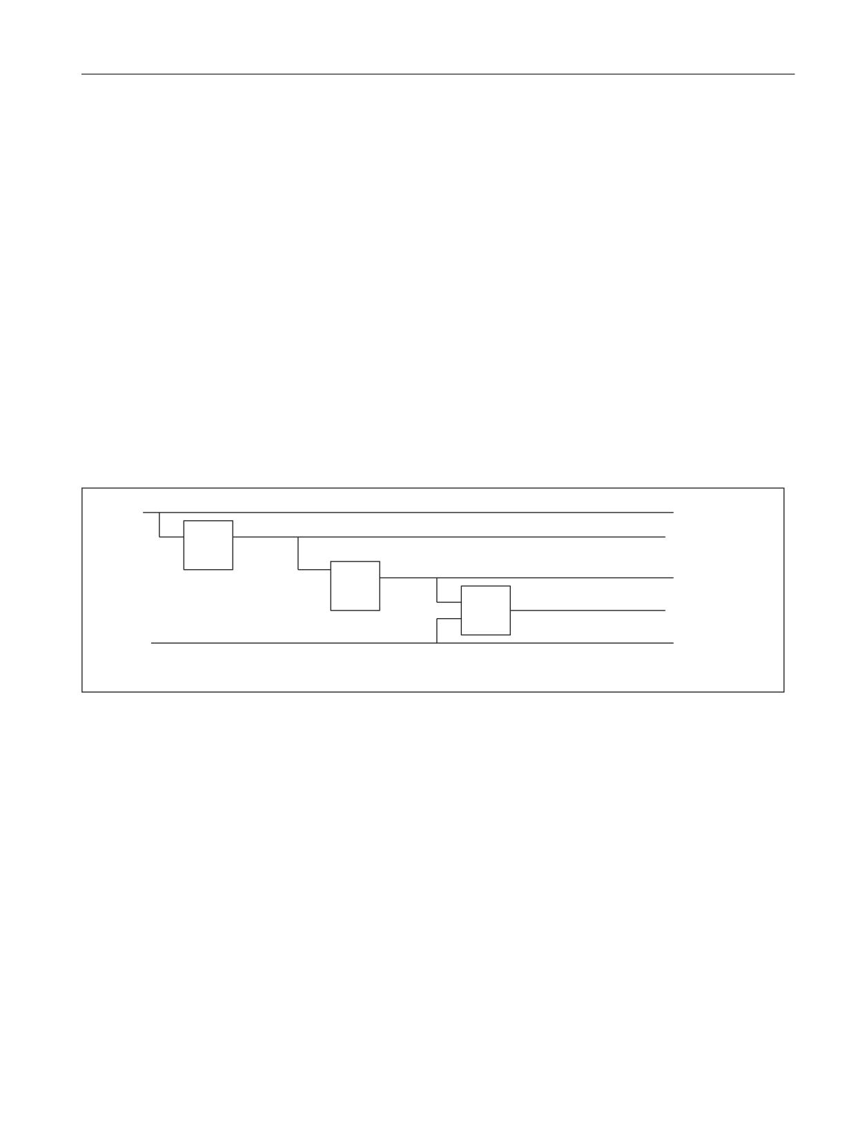
Synchronism difference for EG cascades is the deviation of the actual position of the following
axis from setpoint position that results fro the rule of motion for the real axes involved.
Example:
/$
/$
)$
(*
)$
(*
)$
(*
/$
/$
)$L ൺ )ROORZLQJ D[LV IURP (*L
/$L ൺ UHDO OHDGLQJ D[LV
Figure 10-8
Three-level EG cascade
According to the definition given, the synchronism difference of following axis FA3 in the
example below is determined by the value of following axis FA3Act and the value of leading
axis FA2Act and LA2Act, but not by LA1Act and FA1Act.
If FA2 is not a real axis, the actual value FA2Act is not available. In this case, the setpoint of
the axis derived solely from the leading axis value FA1Act must be used instead of the actual
value of the setpoint of the axis.
Other signals
If an EGON(), EGONSYN() or EGONSYNE() block is encountered in the main run, the signal
"Coupling active" is set for the following axis. If the following axis is only overlaid, the signals
"Coupling active" and "Axis override" are set. If EGON(), EGONSYN() or EGONSYNE() is
active and the following axis is also overlaid, the signals "Coupling active" and "Axis override"
are also set.
IS "following spindle active" DB31, ... DBX 99.1: Coupling active,
IS "overlaid movement" DB31, ... DBX98.4: axis is overlaid,
Special functions
Function Manual, 12/2018, A5E40874099B AB
449
M3: Coupled axes
10.4 Electronic gear (EG)
IS "Enable following axis override" DB31, ... DBX26.4
In the case of the commands EGON() and EGONSYNE(), the "Enable following axis override"
signal must be present for the gear to synchronize to the specified synchronization position
for the following axis. If it is not present, alarm 16771 "Override movement not enabled" is
issued. If the signal is present, the following axis travels to the synchronized position with the
calculated acceleration and at the velocity set for the approach mode.
Further monitoring signals
Machine data MD37550 $MA_EG_VEL_WARNING allows a percentage of the speeds and
accelerations to be specified in the following machine data MD32000 $MA_MAX_AX_VELO
and MD32300 $MA_MAX_AX_ACCEL, with reference to the following axis, which results in
the generation of the following interface signals:
IS "Speed warning threshold" DB31, ... DBX98.5
IS "Acceleration warning threshold" DB31, ... DBX98.6
The monitoring signals can be used as trigger criteria for emergency retraction (see Chapter
"Trigger sources (Page 570)").
Machine data MD37560 $MA_EG_ACC_TOL allows a percentage with reference to machine
data MD32300 $MA_MAX_AX_ACCEL of the following axis to be defined, and the IS signal
"axis accelerates" DB31, ... DBX99.3 to be generated.
Request synchronism difference
1. The result of the synchronism difference calculation can be read as an amount in the part
program with system variable $VA_EG_SYNCDIFF. The relevant value with sign is
available in the system variables $VA_EG_SYNCDIFF_S. The following meanings apply:
● Negative value (in positive traverse direction for lead and following axis): The following axis
lags behind its calculated setpoint position.
● Positive value (in positive traverse direction for lead and following axis): The following axis
leads before its calculated setpoint position (overswing).
The amount of the synchronism difference with sign corresponds to the system variables
without sign from $VA_EG_SYNCDIFF.
$VA_EG_SYNCDIFF[ax] = ABS($VA_EG_SYNCDIFF_S[ax])
Block change mode
1. When an EG axis group is activated, it is possible to specify the conditions under which a
part program block change is to be executed:
2. The specification is made with a string parameter with the following meaning:
3. "NOC": Immediate block change
4. "FINE": Block change if "Fine synchronism" is present
5. "COARSE": Block change if "Coarse synchronism" is present
6. "IPOSTOP": Block change if "Setpoint synchronism" is present
Special functions
450
Function Manual, 12/2018, A5E40874099B AB
M3: Coupled axes
10.4 Electronic gear (EG)
Note
When programmed in activation calls EGON, EGONSYN, EGONSYNE, each of the above
strings can be abbreviated to the first two characters.
If no block change has been defined for the EG axis group and none is currently specified,
"FINE" applies.
10.4.3
Definition of an EG axis group
Note
The following definition commands and switch instructions of the electronic gearbox must all
be contained in only one block of a parts program.
All commands of the electronic gearbox result in a preprocessing stop, except for the activation
commands:
● EGON
● EGONSYN
● EGONSYNE
Definition and activation
The definition described below and activation are separate processes. An activation is not
possible unless it has been defined previously.
Definition of an EG axis group
An EG axis group is defined through the input of the following axis and at least one, but not
more than five, leading axis, each with the relevant coupling type:
EGDEF(following axis, leading axis1, coupling type1, leading axis2, coupling type 2,...)
The coupling type does not need to be the same for all leading axes and must be programmed
separately for each individual leading axis.
Coupling type:
Evaluate actual value of leading axis: 0
Evaluate setpoint of leading axis: 1
The coupling factors are preset to zero when the EG axis group is defined. As such, the group
has no effect on the following axis until it is activated. (See EGON, EGONSYN, EGONSYNE).
Preconditions for defining an EG axis group:
No existing axis coupling may already be defined for the following axis. (If necessary, an
existing axis must be deleted with EGDEL.)
EGDEF triggers preprocessing stop with alarm.
Special functions
Function Manual, 12/2018, A5E40874099B AB
451
M3: Coupled axes
10.4 Electronic gear (EG)
For an example of how to use the EG gearbox for gear hobbing, please see Chapter
"Examples", "Electronic Gearbox for Gear Hobbing".
EGDEF
The gearbox definition with EGDEF should also be used unaltered when one or more leading
axes affect the following axis via a curve table.
The variant extended with the addition of non-linear coupling via curve tables is illustrated in
an extended example in Chapter "Extended Example with non-linear Components".
10.4.4
Activating an EG axis group
Without synchronization
The EG axis group is activated without synchronization selection with:
EGON(FA, block change mode, LA1, Z1, N1, LA2 , Z2, N2,..LA5, Z5, N5.)
The coupling is activated immediately.
With:
FA: Following axis
Depending on block change mode, the next block will be activated:
"NOC": Block change takes place immediately
"FINE": Block change is performed in "Fine synchronism"
"COARSE": Block change is performed in "Coarse synchronism"
"IPOSTOP": Block change is performed for setpoint-based synchronism
LAi: Axis name of the leading axis i
Zi: Counter for coupling factor of leading axis i
Ni: Denominator for coupling factor of leading axis i
Only the leading axes previously specified with the EGDEF command may be programmed in
the activation line. At least one leading axis must be programmed.
The positions of the leading axes and following axis at the instant the grouping is switched on
are stored as "Synchronized positions". The "Synchronized positions" can be read with the
system variable $AA_EG_SYN.
With synchronization
The EG axis group is activated with synchronization selective:
1. EGONSYN
EGONSYN(FA, block change mode, SynPosFA, LAi, SynPosLAi, Z_LAi, N_LAi)
Special functions
452
Function Manual, 12/2018, A5E40874099B AB
M3: Coupled axes
10.4 Electronic gear (EG)
With:
FA: Following axis
Block change mode:
"NOC": Block change takes place immediately
"FINE": Block change is performed in "Fine synchronism"
"COARSE": Block change is performed in "Coarse synchronism"
"IPOSTOP": Block change is performed for setpoint-based synchronism
SynPosFA: Synchronized position of the following axis
LAi: Axis name of the leading axis i
SynPosLAi: Synchronized position of leading axis i
Zi: Counter for coupling factor of leading axis i
Ni: Denominator for coupling factor of leading axis i
Note
The parameters indexed with i must be programmed for at least one leading axis, but for no
more than five.
Only leading axes previously specified with the EGDEF command may be programmed in the
activation line.
Through the programmed "Synchronized positions" for the following axis (SynPosFA) and for
the leading axes (SynPosLA), positions are defined for which the axis grouping is interpreted
as synchronous. If the electronic gear is not in the synchronized state when the grouping is
switched on, the following axis traverses to its defined synchronized position.
The position specification of the synchronized positions is specified in the configured basic
system independently of the programmable dimensions (G70/G71).
If the axis grouping includes modulo axes, their position values are reduced in the modulo,
This way the fastest possible synchronized position is approached reliably, e. g., the next tooth
from the tooth spacing (360 degree* Zn/Ni) and the associated synchronized positions.
(So-called relative synchronization.)
thereby ensuring that they approach the fastest possible synchronized position. (So-called
relative synchronization, e.g. the next tooth gap after "centering".)
If the following interface signal has not been set for the following axis, the axis will not travel
to the synchronization position.
DB31, ... DBX26.4 (Enable following axis override)
Instead the program is stopped at the EGONSYN block and the self-clearing alarm 16771 is
issued until the above mentioned signal is set.
2. EGONSYNE
EGONSYNE(FA, block change mode, SynPosFA, Approach mode, LAi,SynPosLAi, Z_LAi,
N_LAi)
Special functions
Function Manual, 12/2018, A5E40874099B AB
453
M3: Coupled axes
10.4 Electronic gear (EG)
with:
"FA": Following axis
Block change mode:
"NOC": Block change takes place immediately
"FINE": Block change is performed in "Fine synchronism"
"COARSE": Block change is performed in "Coarse synchronism"
"IPOSTOP": Block change is performed for setpoint-based synchronism
SynPosFA: Synchronized position of the following axis
Approach mode:
"NTGT": NextToothGapTime-optimized, the next tooth gap is approached time-optimized
(preset is used if no setting is applied).
"NTGP": The next tooth gap is approached time-optimized.
"ACN": AbsoluteCoordinateNegative, Absolute measurement specification, rotary axis
traverses in negative rotation direction
"ACP": AbsoluteCoordinatePositive, Absolute measurement specification, rotary axis
traverses in positive rotation direction
"DCT": DirectCoordinateTime-optimized, Absolute measurement specification, rotary axis
traverses time-optimized to programmed synchronized position
"DCP": DirectCoordinatePath-optimized, Absolute measurement specification, rotary axis
traverses path-optimized to programmed synchronized position
LAi: Axis name of the leading axis i
SynPosLAi: Synchronized position of leading axis i
Zi: Counter for coupling factor of leading axis i
Ni: Denominator for coupling factor of leading axis i
Note
The parameters indexed with i must be programmed for at least one leading axis, but for no
more than five.
The function is active only for modulo following axes that are coupled to modulo leading axes.
Tooth gap
The tooth gap is defined as 360 degrees * Zi / Ni
Example:
EGONSYNE(A, "FINE", FASysPos, "Traversing mode", B, LASynPos, 2, 10)
Tooth gap: 360*2/10 = 72 (degrees)
Special functions
454
Function Manual, 12/2018, A5E40874099B AB
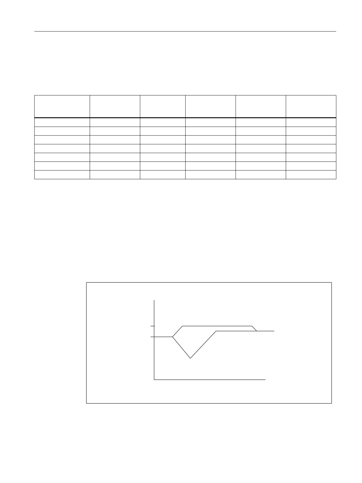
M3: Coupled axes
10.4 Electronic gear (EG)
Approach response with FA at standstill
In this case, the time-optimized and path-optimized traversing modes are identical.
The table below shows the target positions and traversed paths with direction marker (in
brackets) for the particular approach modes:
Programmed
Position of the fol-
Traversing
Traversing mode
Traversing mode
Traversing mode
synchronized posi-
lowing axis before
mode NTGT/
DCT/DCP
ACP
ACN
tion FaSysPos
EGONSYNE
NTGP
110
150
182 (+32)
110 (-40)
110 (+320)
110 (-40)
110
350
326 (-24)
110 (+120)
110 (+120)
110 (-240)
130
0
346 (-14)
130 (+130)
130 (+130)
130 (-230)
130
30
58 (+28)
130 (+100)
130 (+100)
130 (-260)
130
190
202 (+12)
130 (-60)
130 (+300)
130 (-60)
190
0
334 (-26)
190 (-170)
190 (+190)
190 (-170)
230
0
14 (+14)
230 (-130)
230 (+230)
230 (-130)
Approach response for moving FA
The following axis moves at almost maximum velocity in the positive direction when the
coupling is activated by EGONSYNE. The programmed synchronized position of the following
axis is 110, the current position 150. This produces the two alternative synchronized positions
110 and 182 (see table above).
In the case of traversing mode NTGP (path-optimized), synchronized position 182 is selected
independent of the current velocity. This has the shortest distance from the current position of
the following axis. Traversing mode NTGT (time-optimized) considers the current speed of the
following axis and produces a deceleration on account of the limit for the maximum axis speed
to reach synchronism in the shortest possible time (see Figure).
Y
17*3
YPD[
17*7
W
Figure 10-9
Reaching the next tooth gap, FA path-optimized (top) vs. time-optimized (bottom)
Special functions
Function Manual, 12/2018, A5E40874099B AB
455
M3: Coupled axes
10.4 Electronic gear (EG)
Sample notations
EGONSYNE(A, "FINE", 110, "NTGT", B, 0, 2, 10)
couple A to B, synchronized position A = 110, B = 0, coupling factor 2/10, approach mode =
NTGT
EGONSYNE(A, "FINE", 110, "DCT", B, 0, 2, 10)
couple A to B, synchronized position A = 110, B = 0, coupling factor 2/10, approach mode =
DCT
EGONSYNE(A, "FINE", 110, "NTGT", B, 0, 2, 10, Y, 15, 1, 3)
couple A to B, synchronized position A = 110, B = 0, Y = 15,
Coupling factor to B = 2/10, Coupling factor to Y = 1/3,
approach mode = NTGT
With synchronization
The syntax specified above applies with the following different meanings:
If a curve table is used for a leading axis, then the denominator of the linear coupling of the
coupling factor (Ni) must be set to 0 (denominator 0 would be impermissible for linear
couplings).
For control, denominator zero is the indicator that the counter of the coupling factor (Zi) is to
be interpreted as the number of the curve table to be used. The curve table with the specified
number must already be defined at power on (in accordance with Chapter "Curve Tables").
The leading axis specified (LAi) corresponds to the one specified for coupling via coupling
factor (linear coupling).
10.4.5
Deactivating an EG axis group
Variant 1
There are different ways to deactivate an active EG axis grouping.
EGOFS(following axis)
The electronic gear is deactivated. The following axis is braked to a standstill. This call triggers
a preprocessing stop.
Variant 2
The following parameterization of the command makes it possible to selectively control the
influence of individual leading axes on the motion of the following axis.
Special functions
456
Function Manual, 12/2018, A5E40874099B AB
M3: Coupled axes
10.4 Electronic gear (EG)
EGOFS(following axis, leading axis 1, ... leading axis 5)
Note
At least one leading axis must be specified.
The influence of the specified leading axes on the slave is selectively inhibited. This call triggers
a preprocessing stop.
If the call still includes active leading axes, then the slave continues to operate under their
influence. If the influence of all leading axes is excluded by this method, then the following axis
is braked to a standstill.
If the command EGONSYN is deactivated selectively, no axis movement is performed.
Variant 3
EGOFC(following spindle)
The electronic gear is deactivated. The following spindle continues to traverse at the speed/
velocity that applied at the instant of deactivation. This call triggers a preprocessing stop.
Note
Call for following spindles available. For EGOFC a spindle name must be programmed.
10.4.6
Deleting an EG axis group
An EG axis grouping must be switched off, as described in Chapter "Switching off a EG Axis
Group", before its definition can be deleted.
EGDEL(following axis)
The defined coupling of the axis grouping is deleted. Additional axis groups can be defined by
means of EGDEF until the maximum number of simultaneously activated axis groups is
reached.
This call triggers a preprocessing stop.
Special functions
Function Manual, 12/2018, A5E40874099B AB
457

M3: Coupled axes
10.4 Electronic gear (EG)
10.4.7
Interaction between rotation feedrate (G95) and electronic gearbox
The FPR( ) part program command can be used to specify the following axis of an electronic
gear as the axis, which determines the rotational feedrate. The following behavior is applicable
in this case:
● The feedrate is determined by the setpoint velocity of the following axis of the electronic
gear.
● The setpoint velocity is calculated from the speeds of the leading spindles and modulo axes
(which are not path axes) and from their associated coupling factors.
● Velocity components from other leading axes and overlaid motions of the following axis are
not taken into account.
References: /V1/, Feeds
10.4.8
Response to POWER ON, RESET, operating mode change, block search
Function
Behavior regarding electronic gearbox
Coupling state
Configuration
Mode change
Is retained
Is retained
End of part program
Is retained
Is retained
Reset
Is retained
Is retained
Power On 1)
Is not retained
Is not retained
1) No coupling is active after Power On.
Block search
A search while a coupling is active (EG) is possible under the following supplementary
conditions:
● Simulation is exclusively with setpoint coupling.
● No cross-channel leading axes may be disabled.
● Axis movements for which all real positions are known to the NC.
If it is technically not sensible or not possible to permit the target block for a block search with
calculation or SERUPRO within a part program section with active coupling, this section can
be locked for "continue machining at the contour".
Programming
● IPTRLOCK()
● IPTRUNLOCK()
References
(K1) Mode group, channel, program operation, reset response , Section "Block search type 5
SERUPRO" > "Lock program section for continue machining at the contour"
Special functions
458
Function Manual, 12/2018, A5E40874099B AB
M3: Coupled axes
10.4 Electronic gear (EG)
10.4.9
System variables for electronic gearbox
Application
The following system variables can be used in the part program to scan the current states of
an EG axis group and to initiate appropriate reactions if necessary:
Table 10-1
System variables, R means: Read access possible
Name
Type
Access
Preprocessing
Meaning, value
Cond. Index
stop
part
Sync
part pro-
Sync
pro-
act.
gram
act.
gram
$AA_EG_
INT
R
R
Type of coupling:
Axis name
TYPE[a,b]
0: actual value
a: Following axis
1: Setpoint value coupling
b: Leading axis
$AA_EG_
REAL
R
R
Numerator of coupl. factor
Axis name
NUMERA[a,b]
KF
a: Following axis
KF = numerator/denomina-
b: Leading axis
tor
preset: 0
Number of curve table
when $AA_EG_DE-
NOM[a,b] is 0.
$AA_EG_
REAL
R
R
Denominator of coupl. fact.
Axis name
DENOM[a,b]
KF
a: Following axis
KF = numerator/denomina-
b: Leading axis
tor
preset: 1
Denominator must be posi-
tive.
Denominator is 0, if instead
of the numerator
$AA_EG_NUMERA[a,b]
the number of a curve table
is specified.
$AA_EG_
REAL
R
R
Synchronized position for
Axis name
SYN[a,b]
specified leading axis
a: Following axis
Default: 0
b: Leading axis
$AA_EG_
REAL
R
R
Synchronized position for
Axis name
SYNFA[a]
specified following axis
a: Following axis
Default: 0
Special functions
Function Manual, 12/2018, A5E40874099B AB
459
M3: Coupled axes
10.4 Electronic gear (EG)
Name
Type
Access
Preprocessing
Meaning, value
Cond. Index
stop
part
Sync
part pro-
Sync
pro-
act.
gram
act.
gram
$P_EG_BC[a]
STRING
R
R
Block change criterion for
Axis name
EG activation calls: EGON,
a: Following axis
EGONSYN:
"NOC": immediately
"FINE": Synchronoous tra-
verse fine
"COARSE": Synchronous
traverse coarse
"IPOSTOP": Setpoint-
based synchronism
$AA_EG_
INT
R
R
Number of leading axes de-
Axis name
NUM_LA[a]
fined with EGDEF. 0 if no
a: Following axis
axis has been defined as a
following axis with EGDEF.
$AA_EG_
AXIS
R
R
Axis name of leading axis
Axis name
AX[n,a]
whose index n has been
n: Index of leading axis in
specified.
the EG coupling 0 ... 4
a: Following axis
$AA_EG_
BOOL
R
R
Determine power-on state
Axis name
ACTIVE[a,b]
of a leading axis:
a: Following axis
0: Switched off
b: Leading axis
1: activated
$VA_EG_
REAL
R
R
R
Actual value of synchron-
Axis name
SYNCDIFF[a]
ism difference. A compari-
a: Following axis
son of machine data
MD37200 $MA_COU-
PLE_POS_TOL_COARSE
and MD37210 $MA_COU-
PLE_POS_TOL_FINE pro-
duces interface signals.
10.4.10
Examples
10.4.10.1
Example using linear couplings
Use of axes
The following diagram shows the configuration of a typical gear hobbing machine. The machine
comprises five numerically closed loop controlled axes and an open loop controlled main
spindle. These are:
● The rotary motion of the workpiece table (C) and hobbing cutter (B).
● The axial axis (Z) for producing the feed motion over the entire workpiece width.
● The tangential axis (Y) for moving the hobbing cutter along its axis.
Special functions
460
Function Manual, 12/2018, A5E40874099B AB
M3: Coupled axes
10.4 Electronic gear (EG)
● The radial axis (X) for infeeding the cutter to depth of tooth.
● The cutter swivel axis (A) for setting the hobbing cutter in relation to the workpiece as a
function of cutter lead angle and angle of inclination of tooth.
$
=
<
%
;
&
; 5DGLDO D[LV
< 7DQJHQWLDO D[LV PDVWHU GULYH
< 7DQJHQWLDO D[LV PDVWHU GULYH
$ 0LOOLQJ VZLYHO D[LV
& :RUNSLHFH URWDWLRQDO D[LV IROORZLQJ GULYH
% 0LOOLQJ URWDWLRQDO D[LV 0DLQ VSLQGOH 0DLQ GULYH
Figure 10-10
Definition of axes on a gear hobbing machine (example)
The functional interrelationships on the gear hobbing machine are as follows:
%
=
<
/$
/$
/$
:RUNSLHFH ZLGWK
/RQJLWXGLQDO D[LV
RI FXWWHU
5RWDWLRQ RI FXWWHU
&
)$
5RWDU\ D[LV RI ZRUNSLHFH JHDU WRRWK
In this case, the workpiece table axis (C) is the following axis which is influenced by three
master drives.
Special functions
Function Manual, 12/2018, A5E40874099B AB
461
M3: Coupled axes
10.4 Electronic gear (EG)
The setpoint of the following axis is calculated cyclically with the following logic equation:
nc = nb * (z0 / z2) + vz * (udz / z2) + vy * (udy / z2)
with: nc
= Rotational speed of workpiece axis (C)
nb
= Rotational speed of milling spindle (B)
z0
= Number of gears of the hobbing machine
z2
= Number of teeth of the workpiece
vz
= Feed velocity of axial axis (Z)
vy
= Feed velocity of tangential axis (Y)
udz
= Axial differential constant
udy
= Tangential differential constant
Quantities which influence the setpoint of workpiece axis C
The first addend of the above equation determines the speed ratio between workpiece table
and cutter, and thus the number of teeth of the workpiece.
The second addend effects the necessary additional rotation of the C axis as a function of the
axial feed motion of the cutter to produce the tooth inclination on helical teeth.
The third component also makes allowance for additional rotation of the C axis to compensate
for the tangential movement of the cutter in relation to the workpiece, thus ensuring that the
tool is equally stressed over its entire length.
Workpiece/tool parameter
The values z0, z2, udz, and udy are workpiece- or tool-dependent and are specified by the NC
operator or in the part program.
Differential constants
Differential constants udz and udy make allowance for the angle of workpiece teeth and for cutter
geometry. These differential constants can be determined in user-specific cycles.
udz = (sin β° / (mn * π) ) * 360
[degrees/mm]
udy = (cos γ° / (mn * π) ) * 360
[degrees/mm]
with:
mn
= Normal module (in mm)
β°
= Incline angle of gear wheel
γ°
= Pitch angle of hobbing machine
Special functions
462
Function Manual, 12/2018, A5E40874099B AB
M3: Coupled axes
10.4 Electronic gear (EG)
Extract from part program:
Program code
Comment
EGDEF(C,B,1,Z,1,Y,1)
; Definition of EG axis grouping
with setpoint coupling (1) from
B, Z, Y to C (following axis).
EGON(C,"FINE",B,z0,z2,Z,udz,z2,Y,udy,z2)
; Activate coupling.
…
Special functions
Function Manual, 12/2018, A5E40874099B AB
463
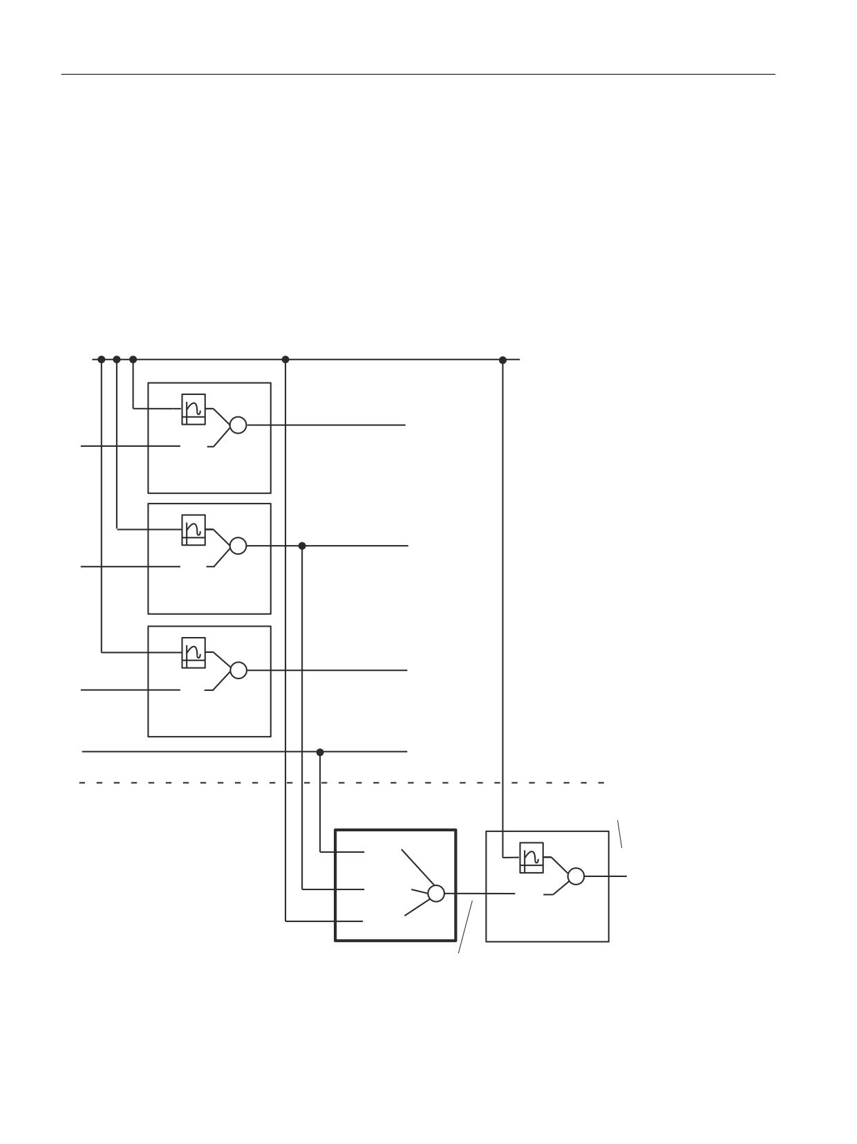
M3: Coupled axes
10.4 Electronic gear (EG)
10.4.10.2
Extended example with non-linear components
Introduction
The following example extends the example (see "Figure 10-10 Definition of axes on a gear
hobbing machine (example) (Page 461)") with the following:
● Machine error compensations which are not linearly dependent on the Z axis, and
● a Z-axis dependent component with tooth geometry.
This can be used to create a slightly convex tooth surface, so that the centre of the tooth
is stressed more than the edges during operation.
/HDGLQJ D[HV
/$
=
=
&
;
=
;
1
*
&
<
<
&RPSHQVDWLRQ I =
=
1
*
&
$
$
=
1
*
%
%
$FFRUGLQJ WR %DVH ([DPSOH
)ROORZLQJ D[LV
=
&
1
&
*HDU JHRPHWU\
=
&
=
2&
1
=
1
*
*
6RIWZDUH D[LV
Figure 10-11
Extended example with non-linear machine fault compensation and non-linear components on the tooth
geometry
Special functions
464
Function Manual, 12/2018, A5E40874099B AB
M3: Coupled axes
10.4 Electronic gear (EG)
The following section of a part program is intended to illustrate the general concept;
supplementary curve tables and gear wheel/machine parameters are still to be added.
Components to be added are marked with <...> . Stated parameters may also have to be
modified, e.g. coupling factors.
Program code
Comment
N100
CTABDEF(X, Z, 1, 0)
; declaration and specification of non-period-
ic curve table C1
N110
<
; Preset of curve table: Curve points or poly-
>
nomial blocks
N190
CTABEND
N200
CTABDEF(Y, Z, 2, 0)
; declaration and specification of non-period-
ic curve table C2
N210
<
; Preset of curve table: Curve points or poly-
>
nomial blocks
N290
CTABEND
N300
CTABDEF(A, Z, 3, 0)
; declaration and specification of non-period-
ic curve table C3
N310
<
; Preset of curve table: Curve points or poly-
>
nomial blocks
N390
CTABEND
N400
CTABDEF(C, Z, 4, 0)
; declaration and specification of non-period-
ic curve table C4
N410
<
; Preset of curve table: Curve points or poly-
>
nomial blocks
N490
CTABEND
N500
EGDEF(X, Z, 1)
; Declaration of path via C1, setpoint coupling
N510
G1 F1000 X10
; declaration of command component of X
N520
EGONSYN(X, "NOC",
; Path switch-on via C1
<SynPosX>, Z,
<SynPosX_Z>, 1, 0)
N600
EGDEF(Y, Z, 1)
; Declaration of path via C2, setpoint coupling
N610
G1 F1000 Y10
; declaration of command component of Y
N620
EGONSYN(Y,
; Path switch-on via C2
"COARSE", <SynPo-
sY>, Z, <SynPo-
sY_Z>, 2, 0)
N700
EGDEF(A, Z, 1)
; Declaration of path via C3, setpoint coupling
N710
G1 F1000 A10
; declaration of command component of A
N720
EGONSYN(A, "FINE",
; Path switch-on via C3
<SynPosA>, Z, <Syn-
PosA_Z>, 3, 0)
; 1. Gear stage, C99 is the software axis between the two electronic gears
N800
EGDEF(C99, Y, 1, Z,
1, B, 1 )
N810
EGONSYN(C99, "NOC",
; Switch-on of leading axis B
<SynPosC99>, B,
<SynPosC99_B>, 18,
2, &
Special functions
Function Manual, 12/2018, A5E40874099B AB
465

M3: Coupled axes
10.4 Electronic gear (EG)
Program code
Comment
Y, <SynPosC99_Y>,
; Switch-on of leading axis Y
R1 * π, 1, &
Z, <SynPosC99_Z>,
; Switch-on of leading axis Z
10, 1)
; "&" character means: command continued in
next line, no LF nor comment permissible in
program
; 2. Gear stage
N900
EGDEF(C, C99, 1, Z,
; declaration of following C99 of step 1 as
1)
leading axis of step 2,
; Setpoint value coupling
N910
; Declaration of path via C4, setpoint cou-
pling
N920
EGONSYN(C, "NOC",
; Switch-on of software axis C99
<SynPosC>, C99,
<SynPosC_C99>, 1,
1, &
Z, <SynPosC_Z>, 4,
; and of leading axis Z via C4
0)
N999
M30
Machine data
Only one section is specified, which extends beyond the necessary geometry/channel
configuration and machine axis parameters.
$MN_NUM_EG = 5
; Maximum number of gearboxes
$MN_MM_NUM_CURVE_TABS = 5
; Maximum number of curve tables
$MN_MM_NUM_CURVE_SEGMENTS = 50
; Maximum number of curve segments
$MN_MM_NUM_CURVE_POLYNOMS = 100
; Maximum number of curve polynomials
Setting data
If the scaling described in Section "Electronic gear (EG) (Page 442) is used, the function value
from the following machine data changes according to the displacement:
MD43108 $SD_LEAD_SCALE_OUT_POS[4] = 1.2 ; scaling for table C4
System variables
In accordance with the above definitions, the following values are entered in the associated
system variables by the control.
Reference:
List Manual, System Variables
Special functions
466
Function Manual, 12/2018, A5E40874099B AB
M3: Coupled axes
10.4 Electronic gear (EG)
The system variables listed below are only used for explanatory purposes!
; ************** Gear X (G1)
$AA_EG_TYPE[X, Z] = 1
; Setpoint value coupling
$AA_EG_NUMERA[X, Z] = 1
; curve table No. = 1
$AA_EG_DENOM[X, Z] = 0
; nominator = 0 → curve table applies
$P_EG_BC[X] = "NOC"
; Block change criterion
$AA_EG_NUM_LA[X] = 1
; Number of leading axes
$AA_EG_AX[0, X] = Z
; name of leading axis
$AA_EG_SYN[X,Z] = <SynPosX_Z>
; Synchronized position of leading axis Z
$AA_EG_SYNFA[X] = <SynPosX>
; Synchronized position of the following axis
; ************** Gear Y (G2)
$AA_EG_TYPE[Y, Z] = 1
; Setpoint value coupling
$AA_EG_NUMERA[Y, Z] = 2
; curve table No. = 2
$AA_EG_DENOM[Y, Z] = 0
; nominator = 0 → curve table applies
$P_EG_BC[Y10] = "COARSE"
; Block change criterion
$AA_EG_NUM_LA[Y] = 1
; Number of leading axes
$AA_EG_AX[0, Y] = Z
; name of leading axis
$AA_EG_SYN[Y, Z] = <SynPosY_Z>
; Synchronized position of leading axis Z
$AA_EG_SYNFA[Y] = <SynPosY>
; Synchronized position of the following axis
; ************** Gear A (G3)
$AA_EG_TYPE[A, Z] = 1
; Setpoint value coupling
$AA_EG_NUMERA[A, Z] = 3
; curve table No. = 3
$AA_EG_DENOM[A, Z] = 0
; nominator = 0 → curve table applies
$P_EG_BC[A10] = "FINE"
; Block change criterion
$AA_EG_NUM_LA[A] = 1
; Number of leading axes
$AA_EG_AX[0, A] = Z
; name of leading axis
$AA_EG_SYN[A, Z] = <SynPosA_Z>
; Synchronized position of leading axis Z
$AA_EG_SYNFA[A] = <SynPosA>
; Synchronized position of the following axis
; ************** Gear C99 (G4)
$AA_EG_TYPE[C99, Y] = 1
; Setpoint value coupling
$AA_EG_NUMERA[C99, Y] = 18
; numerator for coupling factory
$AA_EG_DENOM[C99, Y] = 2
; denominator for coupling factory
$AA_EG_TYPE[C99, Z] = 1
; Setpoint value coupling
$AA_EG_NUMERA[C99, Z] = R1 * π
; numerator for coupling factorz
$AA_EG_DENOM[C99, Z] = 1
; denominator for coupling factorz
$AA_EG_TYPE[C99, B] = 1
; Setpoint value coupling
$AA_EG_NUMERA[C99, B] = 10
; numerator for coupling factorb
$AA_EG_DENOM[C99, B] = 1
; denominator for coupling factorb
$P_EG_BC[C99] = "NOC"
; Block change criterion
$AA_EG_NUM_LA[C99] = 3
; Number of leading axes
$AA_EG_AX[0, C99] = Y
; name of leading axis Y
$AA_EG_AX[1, C99] = Z
; name of leading axis Z
Special functions
Function Manual, 12/2018, A5E40874099B AB
467
M3: Coupled axes
10.4 Electronic gear (EG)
$AA_EG_AX[2, C99] = B
; name of leading axis B
$AA_EG_SYN[C99, Y] = <SynPosC99_Y>
; Synchronized position of leading axis Y
$AA_EG_SYN[C99, Z] = <SynPosC99_Z>
; Synchronized position of leading axis Z
$AA_EG_SYN[C99, B] = <SynPosC99_B>
; Synchronized position of leading axis B
$AA_EG_SYNFA[C99] = <SynPosC99>
; Synchronized position of the following axis
; *************** Gear C (G5)
$AA_EG_TYPE[C, Z] = 1
; Setpoint value coupling
$AA_EG_NUMERA[C, Z] = 4
; curve table No. = 4
$AA_EG_DENOM[C, Z] = 0
; nominator = 0 → curve table applies
$AA_EG_TYPE[C, C99] = 1
; Setpoint value coupling
$AA_EG_NUMERA[C, C99] = 1
; numerator for coupling factorC99
$AA_EG_DENOM[C, C99] = 1
; denominator for coupling factorC99
$P_EG_BC[C] = "NOC"
; Block change criterion
$AA_EG_NUM_LA[C] = 2
; Number of leading axes
$AA_EG_AX[0, C] = Z
; name of leading axis Z
$AA_EG_AX[1, C] = C99
; name of leading axis C99
$AA_EG_SYN[C, Z] = <SynPosC_Z>
; Synchronized position of leading axis Z
$AA_EG_SYN[C, C99] = <SynPosC_C99>
; Synchronized position of leading axis C99
$AA_EG_SYNFA[C] = <SynPosC>
; Synchronized position of leading axis C
Machine data
Extract from MD:
; ************** Channel 1
CHANDATA(1)
; ************** Axis 1, "X"
$MC_AXCONF_GEOAX_NAME_TAB[0] = "X"
$MC_AXCONF_CHANAX_NAME_TAB[0] = "X"
$MC_AXCONF_MACHAX_USED[0]=1
$MN_AXCONF_MACHAX_NAME_TAB[0] = "X1"
$MA_SPIND_ASSIGN_TO_MACHAX[AX1] = 0
$MA_IS_ROT_AX[AX1] = FALSE
; *************** Axis 2, "Y"
$MC_AXCONF_GEOAX_NAME_TAB[1]="Y"
$MC_AXCONF_CHANAX_NAME_TAB[1] = "Y"
$MC_AXCONF_MACHAX_USED[1] = 2
$MN_AXCONF_MACHAX_NAME_TAB[1] = "Y1"
$MA_SPIND_ASSIGN_TO_MACHAX[AX2] = 0
$MA_IS_ROT_AX[AX2] = FALSE
Special functions
468
Function Manual, 12/2018, A5E40874099B AB
M3: Coupled axes
10.4 Electronic gear (EG)
; *************** Axis 3, "Z"
$MC_AXCONF_GEOAX_NAME_TAB[2] = "Z"
$MC_AXCONF_CHANAX_NAME_TAB[2] = "Z"
$MC_AXCONF_MACHAX_USED[2]=3
$MN_AXCONF_MACHAX_NAME_TAB[2] = "Z1"
$MA_SPIND_ASSIGN_TO_MACHAX[AX3] = 0
$MA_IS_ROT_AX[AX3] = FALSE
; *************** Axis 4, "A"
$MC_AXCONF_CHANAX_NAME_TAB[3] = "A"
$MC_AXCONF_MACHAX_USED[3]=4
$MN_AXCONF_MACHAX_NAME_TAB[3] = "A1"
$MA_SPIND_ASSIGN_TO_MACHAX[AX4]=0
$MA_IS_ROT_AX[AX4] = TRUE
$MA_ROT_IS_MODULO[AX4] = TRUE
; *************** Axis 5, "B"
$MC_AXCONF_CHANAX_NAME_TAB[4] = "B"
$MC_AXCONF_MACHAX_USED[4]=5
$MC_SPIND_DEF_MASTER_SPIND = 1
$MN_AXCONF_MACHAX_NAME_TAB[4] = "B1"
$MA_SPIND_ASSIGN_TO_MACHAX[AX5] = 1
$MA_IS_ROT_AX[AX5] = TRUE
$MA_ROT_IS_MODULO[AX5] = TRUE
; ************** Axis 6, "C"
$MC_AXCONF_CHANAX_NAME_TAB[5] = "C"
$MC_AXCONF_MACHAX_USED[5]=6
$MN_AXCONF_MACHAX_NAME_TAB[5] = "C1"
$MA_SPIND_ASSIGN_TO_MACHAX[AX6] = 0
$MA_IS_ROT_AX[AX6] = TRUE
$MA_ROT_IS_MODULO[AX6] = TRUE
; ************** Axis 10, "C99"
$MC_AXCONF_CHANAX_NAME_TAB[9] = "C99"
$MC_AXCONF_MACHAX_USED[9]=10
$MA_SPIND_ASSIGN_TO_MACHAX[AX10] = 0
$MA_IS_ROT_AX[AX10] = TRUE
$MA_ROT_IS_MODULO[AX10] = TRUE
Special functions
Function Manual, 12/2018, A5E40874099B AB
469
M3: Coupled axes
10.5 Generic coupling
10.5
Generic coupling
10.5.1
Brief description
10.5.1.1
Function
Function
"Generic Coupling" is a general coupling function, combining all coupling characteristics of
existing coupling types (coupled motion, master value coupling, electronic gearbox and
synchronous spindle).
The function allows flexible programming:
● Users can select the coupling properties required for their applications (building block
principle).
● Each coupling property can be programmed individually.
● The coupling properties of a defined coupling (e.g. coupling factor) can be changed.
● Later use of additional coupling properties is possible.
● The coordinate reference system of the following axis (Base co-ordinate system or Machine
co-ordinate system) is programmable.
● Certain coupling properties can also be programmed with synchronous actions.
References:
Function Manual, Synchronized Actions
Adaptive cycles
Previous coupling calls for coupled motion (TRAIL*), Master value coupling (LEAD*), Electronic
Gearbox (EG*) and Synchronous spindle (COUP*) are still supported via adaptive cycles (see
Section "Adaptive cycles (Page 520)").
10.5.1.2
Requirements
CP version
The generic coupling is available in a basic version and four optional versions:
● CP-STATIC
● CP-BASIC
● CP-COMFORT
● CP-EXPERT
Special functions
470
Function Manual, 12/2018, A5E40874099B AB
M3: Coupled axes
10.5 Generic coupling
This structure is based on the following considerations:
● Functional scope and required application knowledge increase from the basic version to
the optional CP_EXPERT version.
● The number of required couplings (following axes, following spindles) and their properties
are decisive in the selection of versions.
- Example of simultaneous operation:
If sequential operation of 1 x synchronous spindle pair for part transfer from the main to
the supplementary spindle and the 1 x multi-edge turning is required, then the CP-BASIC
option is suitable and sufficient. However, if it cannot be excluded that both operations
can overlap (multi-edge turning running when part transfer is started), the CP-
COMFORT option would be required.
- Example of property:
If a coupled axis grouping with a leading axis is required, the base version is sufficient.
For coupled motion groups with two leading axes, one of the optional versions is
required.
● Individual versions are independent of each other. They can be combined and can be
activated simultaneously.
Table 10-2
Quantity structure, which is dependent on the execution of coupling modules that can be simultaneously activated
Typ
CP versions allow one or more different CPSETTYPE
Base ver-
CP-
CP-BA-
CP-COM-
CP-EX-
e
coupling objects simultaneously:
sion
STATIC
SIC
FORT
PERT
A
Coupled motion
4
-
4
4
8
B
Synchronous spindle with |1|:1 coupling
-
1
-
-
-
C
o./u. Synchronous spindles, multi-edge turning
-
-
1
4
8
o./u. Master value coupling / curve tables interpolation
o./u. MCS coupling
D
o./u. Electronic gearbox "plain"
-
-
-
1
8
o./u. Free generic coupling "basic"
E
o./u. Electronic gear
-
-
-
-
5
o./u. Free generic coupling
o./u. stands for over/under
Table 10-3
Scaling of availability of coupling properties
Type A
Type B
Type C
Type D
Type E
20
1
13
9
5
Maximum number of CPSETTYPE-related functionalities (per
type)
TRAIL - coupled motion
20
-
13
9
5
Maximum number of coupled motion groups with the following
properties:
→ refer to CPSETTYPE="TRAIL"1)
1
2
2
2
Maximum number of master values
-
-
+
+
Coupling between a spindle and an axis
Special functions
Function Manual, 12/2018, A5E40874099B AB
471

M3: Coupled axes
10.5 Generic coupling
Type A
Type B
Type C
Type D
Type E
+
+
+
+
Coupling between a rotary axis and a linear axis
-
+
+
+
From part program and synchronous actions
+
+
+
+
Superimposition / speed difference permitted
-
-
-
+
Cascading permitted
BCS
BCS /
BCS /
BCS /
Coordinate reference (default): CPFRS="BCS")
MCS
MCS
MCS
Synchronous spindle with |1|:1 coupling
-
1
-
-
-
Maximum number of synchronous spindles / multi-edge turning
with the following properties:
→ refer to CPSETTYPE="COUP"1)
1
Maximum number of master values
-
From part program and synchronous actions
-
Superimposition / speed difference permitted
-
Cascading permitted
MCS
Coordinate reference fix (CPFRS="MCS")
COUP - synchronous spindle/multi-edge turning
-
-
13
9
5
Maximum number of synchronous spindles / multi-edge turning
with the following properties:
→ refer to CPSETTYPE="COUP"1)
1
1
1
Maximum number of master values
-
-
-
From part program and synchronous actions
+
+
+
Superimposition / speed difference permitted
-
-
-
Cascading permitted
MCS
MCS
MCS
Coordinate reference fix (CPFRS="MCS")
LEAD - master value coupling / curve tables interpolation
-
-
13
9
5
Maximum number of master value couplings / curve tables inter-
polation with the following properties:
→ refer to CPSETTYPE="LEAD"1)
1
1
1
Maximum number of master values
+
+
+
From part program and synchronous actions
+
+
+
Superimposition / speed difference permitted
-
-
+
Cascading permitted
BCS /
BCS /
BCS /
Coordinate reference (default): CPFRS="BCS")
MCS
MCS
MCS
EG - electronic gearbox
-
-
-
9
5
Maximum number of electronic gearboxes
with the following properties:
→ refer to CPSETTYPE="EG"1)
3
5
Maximum number of master values
-
-
From part program and synchronous actions
+
+
Superimposition / speed difference permitted
-
+
Cascading permitted
BCS /
BCS /
Coordinate reference (default): CPFRS="BCS")
MCS
MCS
Special functions
472
Function Manual, 12/2018, A5E40874099B AB
M3: Coupled axes
10.5 Generic coupling
Type A
Type B
Type C
Type D
Type E
-
+
Non-linear coupling law (CPLCTID) permitted
CP - free generic coupling
-
-
-
9
5
Maximum number of free generic couplings
with the following properties:
Default (corresponds to CPSETTYPE="CP"1))
3
5
Maximum number of master values
+
+
From part program and synchronous actions
+
+
Superimposition / speed difference permitted
-
+
Cascading permitted
BCS /
BCS /
Coordinate reference (default): CPFRS="BCS")
MCS
MCS
-
+
Non-linear coupling law (CPLCTID) permitted
1) Refer to " Coupling types (CPSETTYPE) (Page 521) ".
Note
Existing coupling options (Master value coupling, Electronic gearbox and Synchronous
spindle) are not taken into consideration by generic coupling. Simultaneous operation of
existing coupling options and generic coupling is only possible if the couplings refer to different
axes/spindles.
Memory configuration
Memory space reserved in dynamic NC memory for generic coupling is defined in machine
data:
MD18450 $MN_MM_NUM_CP_MODULES (maximum allowed number of CP coupling
modules)
MD18452 $MN_MM_NUM_CP_MODUL_LEAD (maximum allowed number of CP master
values)
Note
Recommendation: Expected maximum values, which can be expected simultaneously for this
machine in its maximum configuration, should already be set during commissioning.
Hardware requirements
Systems with more than 6 axes are required when using the "CP-EXPERT" option.
Special functions
Function Manual, 12/2018, A5E40874099B AB
473
M3: Coupled axes
10.5 Generic coupling
10.5.2
Fundamentals
10.5.2.1
Coupling module
With the help of a coupling module, the motion of one axis (→ following axis) can be interpolated
depending on other axes (→ leading axes).
Coupling rule
The relationships between leading axis/values and a following axis are defined by a coupling
rule (coupling factor or curve table). The individual motion components from the individual
leading axes/values have an additive effect.
The relationship is demonstrated by the following example (following axis with two leading
axes):
&RXSOLQJ UXOH
/HDGLQJ D[LV
/$
.)
&RXSOLQJ UXOH
/HDGLQJ D[LV
/$
.)
)$'HS
)$'HS
)ROORZLQJ D[LV
)$&PG
)$7RWDO
FATotal
Total setpoint value of the following axis
FACmd
Setpoint value set in part program
= independent motion component of the following axis
FADEP1
Dependent motion component of leading axis 1
FADEP2
Dependent motion component of leading axis 2
LA1
Setpoint or actual value of the 1st leading axis
LA2
Setpoint or actual value of the 2nd leading axis
SynPosLA1
Synchronized position of the 1st leading axis
SynPosLA2
Synchronized position of the 2nd leading axis
KF1
Coupling factor of the 1st leading axis
KF2
Coupling factor of the 2nd leading axis
Special functions
474
Function Manual, 12/2018, A5E40874099B AB
M3: Coupled axes
10.5 Generic coupling
The following axis position results from the overlay (summation) of the dependent motion
components (FADEP1 and FADEP2), which result from the individual coupling relationships to the
leading axes, and of the independent motion component (FACmd) of the following axis:
FATotal = FACmd + FADEP1 + FADEP2
The motion components of the following axis are calculated as follows:
Dependent motion component of leading axis 1:
FADEP1 = (LA1 - SynPosLA1) * KF1
Dependent motion component of leading axis 2:
FADEP2 = (LA2 -SynPosLA2) * KF2
Independent motion component of the following axis:
FACmd
Following axis overlay
The overlay of dependent and independent motion components of the following axis is called
following axis overlay.
The independent motion component of the following axis can be programmed with the full
range of available motion commands.
10.5.2.2
Keywords and coupling characteristics
Keywords
Programming is done via language commands, e.g. coupled motion with TRAILON(X,Y,2).
Keywords replace the language commands in generic coupling.
This has the following advantages:
● Coupling characteristics can be programmed individually (see following example).
● Programming of multiple couplings can be done in one block (since keywords do not require
their own block).
Advantage: Reduction of work off time
Example:
The properties set with the existing coupling call TRAILON(X,Y,2)(following axis, leading
axis and coupling factor) are defined in the generic coupling with the following keywords:
CPON=(X1) CPLA[X1]=(X2) CPLNUM[X1,X2]=2
CPON=(X1)
Switch on coupling to following axis X1.
CPLA[X1]=(X2)
Define axis X2 as leading axis.
CPLNUM[X1,X2]=2
Set numerator of the coupling factor to 2.
Notation
Special functions
Function Manual, 12/2018, A5E40874099B AB
475

M3: Coupled axes
10.5 Generic coupling
In order to be uniquely assigned, keywords are furnished with the prefix "CP", for Coupling).
Depending on meaning and application position, a third letter is used:
Keyword prefix
Meaning
Example
CP*
Describes the characteristics of the entire coupling.
CPON1)
CPF*
Describes the characteristics of the following axis (Fol-
CPFPOS1)
lowing axis).
CPL*
Describes a property referring to the leading axis (Lead-
CPLON1),
ing axis) or the coupling rule.
CPLNUM1)
CPM*
Describes a property of the entire coupling for special
CPMRESET1)
states.
1) For keyword meaning, please refer to the following table "Overview of all keywords and coupling
characteristics".
Overview of all keywords and coupling characteristics
The following table gives an overview of all keywords of the generic coupling and the
programmable coupling characteristics:
Keyword
Coupling characteristics / meaning
Default setting (CPSET-
TYPE="CP")
CPDEF
Creating a coupling module
CPDEL
Deletion of a coupling module
CPLDEF
Definition of a leading axis and creation of a coupling
module
CPLDEL
Deleting a leading axis of a coupling module
CPON
Switching on a coupling module
CPOF
Switching off a coupling module
CPLON
Switching on a leading axis of a coupling module
CPLOF
Switching off a leading axis of a coupling module
CPLNUM
Numerator of the coupling factor
1.0
CPLDEN
Denominator of the coupling factor
1.0
CPLCTID
Number of curve table
Not set
CPLSETVAL
Coupling reference
CMDPOS
CPFRS
Co-ordinate reference system
BCS
CPBC
Block change criterion
NOC
CPFPOS + CPON
Synchronized position of the following axis when
Not set
switching on
CPLPOS + CPON
Synchronized position of the leading axis when
Not set
switching on
CPFMSON
Synchronization mode
CFAST
CPFMON
Behavior of the following axis at switching on
STOP
Special functions
476
Function Manual, 12/2018, A5E40874099B AB
M3: Coupled axes
10.5 Generic coupling
Keyword
Coupling characteristics / meaning
Default setting (CPSET-
TYPE="CP")
CPFMOF
Behavior of the following axis at complete switch-off
STOP
CPFPOS + CPOF
Switch-off position of the following axis when switch-
Not set
ing off
CPMRESET
Coupling response to RESET
NONE
CPMSTART
Coupling behavior at part program start
NONE
CPMPRT
Coupling response when the part program starts un-
NONE
der block search run via program test
CPLINTR
Offset value of the input value of a leading axis
0.0
CPLINSC
Scaling factor of the input value of a leading axis
1.0
CPLOUTTR
Offset value for the output value of a coupling
0.0
CPLOUTSC
Scaling factor for the output value of a coupling
1.0
CPSYNCOP
Threshold value of position synchronism "Coarse"
MD37200
CPSYNFIP
Threshold value of position synchronism "Fine"
MD37210
CPSYNCOP2
Second threshold value for the "Coarse" position
MD37202
synchronism
CPSYNFIP2
Second threshold value for the "Fine" position syn-
MD37212
chronism
CPSYNCOV
Threshold value of velocity synchronism "Coarse"
MD37220
CPSYNFIV
Threshold value of velocity synchronism "Fine"
MD37230
CPMBRAKE
Response of the following axis to certain stop signals
1
and stop commands
CPMVDI
Response of the following axis to certain NC/PLC
0 (for bits 0 to 3, 5)
interface signals
1 (for bits 4, 6)
CPMALARM
Suppression of special coupling-related alarm out-
MD11410
puts
MD11415
CPSETTYPE
Coupling type
CP
Note
Coupling characteristics, which are not explicitly programmed (in part program of synchronous
actions), become effective with their default settings (see right hand column of the table).
Depending on the settings of the keyword CPSETTYPE instead of the default settings
(CPSETTYPE="CP") preset coupling characteristics can become effective (see Section
"Coupling types (Page 521)").
Special functions
Function Manual, 12/2018, A5E40874099B AB
477

M3: Coupled axes
10.5 Generic coupling
10.5.2.3
System variables
The current state of a coupling characteristic set with a keyword, can be read and written to
with the relevant system variable.
Note
When writing in the part program, PREPROCESSING STOP is generated.
Notation
The names of system variables are normally derived from the relevant keywords and a
corresponding prefix.
The first letter of the prefix defines the access location when reading:
System variable prefix
Access location during read
Features
$PA_CP
Reading of channel referenced axis
Use in synchronous actions is not
specific coupling characteristics in
possible.
block preparation (Preparation)
Does not generate an implicit pre-
processing stop.
$AA_CP
Reading of the current state of the
Use in the part program and in syn-
coupling module (across channels).
chronous actions is possible.
Generates an implicit preprocess-
ing stop when used in the part pro-
gram.
Note
The preprocessing value of a $PA_CP.. CP system variable only differs from the values of the
corresponding $AA_CP.. CP system variable during active part program processing.
At the end of the program or with abort, there is an appropriate synchronization of the
preprocessing with the main run states.
System variable list
A list of all system variables which can be used in a generic coupling is contained in the data
lists (see Section "System variables (Page 553)").
For a detailed description of system variables, refer to:
Reference:
Parameter Manual, System Variables
10.5.3
Creating/deleting coupling modules
10.5.3.1
Creating a coupling module (CPDEF)
An axial coupling module is created through the definition of the following axis.
Special functions
478
Function Manual, 12/2018, A5E40874099B AB