SINUMERIK 840D sl. Service - Functions. Manual (2018-2020)

Acceleration and jerk

4.2 Detailed description

Note

When calculating the limitation value, the value of SD42500 $SC_SD_MAX_PATH_ACCEL is only

taken into account if SD42502 $SC_IS_SD_MAX_PATH_ACCEL is set to "TRUE".

If both PACCLIM and SD42500 $SC_SD_MAX_PATH_ACCEL are active, the smaller of the two

limitation values becomes effective.

Example

Program code

Comment

N1000 G0 X0 Y0 F10000 G64 G710

N1100 G1 X20 RNDM=5

N1200 G1 Y20 PACCLIM=0.5

; The axis slide in Y direction is accel-

erated/decelerated at max. 0.5 m/ss.

N1300 G1 X0 Y40

; The path movement of the axis slides in

X direction and Y direction is acceler-

ated/decelerated at max. 0.5 m/ss.

N1400 G1 Y0

M30

4.2.7

Path acceleration for real-time events (channel-specific)

4.2.7.1

Function

So that no compromise has to be made between machining-optimized acceleration on the one

hand and time-optimized acceleration in connection with the following real-time events on the

other:

• NC Stop / NC Start

• Changing the feedrate override

• Changing the velocity default for "safely reduced velocity" within the context of the "Safety

Integrated" function

For the real-time events mentioned above, the path acceleration can be specified using a

channel-specific system variable:

$AC_PATHACC = path acceleration

Real-time event acceleration will only be active for the duration of the change in velocity in

respect of one of the real-time events specified above.

Axes and spindles

Function Manual, 10/2020, 6FC5397-4GP40-0BA1

Acceleration and jerk

4.2 Detailed description

Limitation

If the specified path acceleration exceeds the capabilities of the machine axes that are of

relevance for the path, a limit will be imposed on the path acceleration within the controller so

that the resulting axial acceleration (a_res) is restricted to less than 2x the parameterized

maximum axial value (a_max).

a_res = 2 * a_max,with a_max = MD32300 $MA_MAX_AX_ACCEL

Note

Path acceleration for real-time events is enabled, irrespective of the radial acceleration.

Effectiveness

Effective

Real-time event acceleration is only enabled in AUTOMATIC and MDA operating modes in

conjunction with the following real-time events:

• NC Stop / NC Start

• Override changes

• Changing the velocity default for "safely reduced velocity" within the context of the

"Safety Integrated" function

Not effective

Path acceleration for real-time events is ineffective for changes in path velocity that are

attributable to path planning during preprocessing for the channel, such as contour

curvatures, corners, kinematic transformation limitations, etc.

Real-time-event path acceleration is ineffective if the programmed value is smaller than

the path acceleration calculated during preprocessing for the path section concerned.

Programming

For information about programming system variables in the part program or synchronized

actions, see Section "Programming (Page 91)".

4.2.7.2

Programming

Syntax

$AC_PATHACC = path acceleration

Functionality

Real-time-event path acceleration is set via the channel-specific system variables.

Parameter: Path acceleration

• Value range: Path acceleration ≥ 0

• Unit: m/s²

Deactivation: $AC_PATHACC = 0

Axes and spindles

Function Manual, 10/2020, 6FC5397-4GP40-0BA1

Acceleration and jerk

4.2 Detailed description

Application:

• Part program

• Static synchronized action

Reset response

Real-time-event path acceleration is deactivated on reset.

Supplementary conditions

Programming $AC_PATHACC in the part program automatically triggers a preprocessing stop

with REORG (STOPRE).

4.2.8

Acceleration with programmed rapid traverse (G00) (axis-specific)

4.2.8.1

Function

Frequently the acceleration for the machine axes participating in processing must be set lower

than that which corresponds to the performance capability of the machine, due to the

processing-specific constraints.

For time-optimized traversing of the machine axes for programmed rapid traverse (part program

instruction G00), a separate maximum value of the axis-specific acceleration can be

parameterized.

JOG setup mode

The acceleration during rapid traverse override (ROV) in JOG setup mode is not affected by this

functionality.

4.2.8.2

Parameterization

The maximum value for axis-specific acceleration with programmed rapid traverse is

parameterized (G00) using the axis-specific machine data:

MD32434 $MA_G00_ACCEL_FACTOR

(scaling of the acceleration limitation with G00)

This is used to generate the maximum value for axis-specific acceleration with programmed

rapid traverse (G00) that is taken into account by the path planning component during

preprocessing:

Acceleration[axis] =

MD32300 $MA_MAX_AX_ACCEL * MD32434 $MA_G00_ACCEL_FACTOR

Axes and spindles

Function Manual, 10/2020, 6FC5397-4GP40-0BA1

Acceleration and jerk

4.2 Detailed description

4.2.9

Acceleration with active jerk limitation (SOFT/SOFTA) (axis-specific)

4.2.9.1

Function

When accelerating with jerk limitation, with the same maximum acceleration value a certain

time loss arises compared with acceleration without jerk limitation. To compensate for this loss

of time, a separate maximum value of the axis-specific acceleration can be parameterized for the

traversing of the machine axes when jerk limiting is active (SOFT/SOFTA).

The maximum value for acceleration with active jerk limitation is parameterized via a factor

relating to the axis-specific maximum value. This results in the maximum value of the axis-

specific acceleration with active jerk limiting that is taken into account by the path planning

component during preprocessing:

Acceleration[<axis>] =

MD32300 $MA_MAX_AX_ACCEL * MD32433 $MA_SOFT_ACCEL_FACTOR

4.2.9.2

Parameterization

The maximum value for acceleration with active jerk limitation (SOFT/SOFTA) is parameterized

using the axis-specific machine data:

MD32434 $MA_SOFT_ACCEL_FACTOR

(scaling of the acceleration limitation with SOFT)

4.2.10

Exceeding the acceleration with non-tangential block transitions (axis-

specific)

4.2.10.1

Function

In the case of non-tangential block transitions (corners), the controller may have to decelerate

the traversing motion of the geometry axes significantly to ensure compliance with the

parameterized axis dynamics. To reduce or prevent the deceleration at non-tangential block

transitions, a higher axis-specific acceleration can be allowed.

The exceeded acceleration is parameterized via a factor relating to the axis-specific maximum

value. This results in the maximum value of the axis-specific acceleration for non-tangential

block transitions that is taken into account by the path planning during preprocessing:

Acceleration[axis] =

MD32300 $MA_MAX_AX_ACCEL * MD32310 $MA_MAX_ACCEL_OVL_FACTOR

4.2.10.2

Parameterization

Excessive acceleration for non-tangential block transitions is parameterized using the axis-

specific machine data:

MD32310 $MA_MAX_ACCEL_OVL_FACTOR

(overload factor for velocity jumps)

Axes and spindles

Function Manual, 10/2020, 6FC5397-4GP40-0BA1

Acceleration and jerk

4.2 Detailed description

4.2.11

Acceleration reserve for the radial acceleration (channel-specific)

4.2.11.1

Function

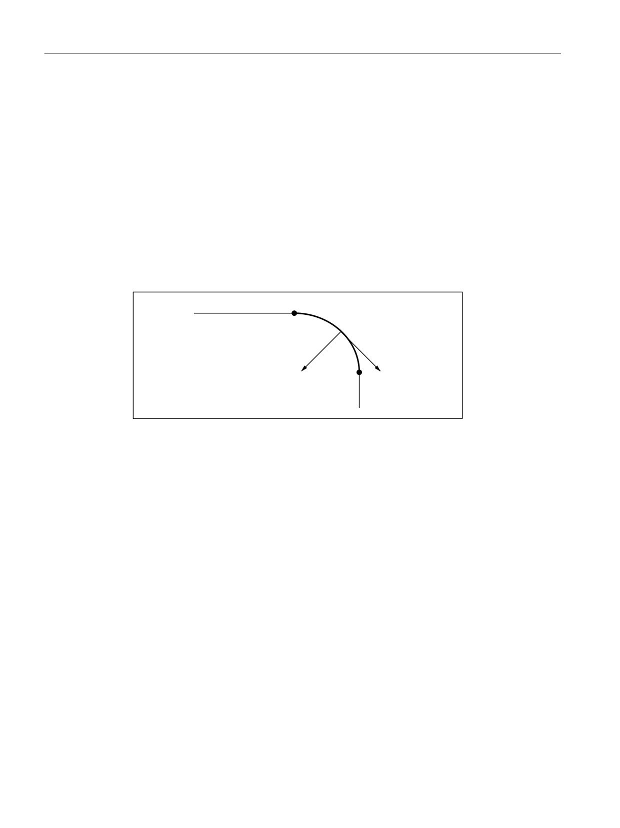
In addition to the path acceleration (tangential acceleration), the radial acceleration also affects

curved contours. If this is not taken into consideration during the parameterization, the active

axial acceleration during acceleration or deceleration on the curved contour can be up to 2 times

the maximum value for a short time.

Active axial acceleration =

portion of the path acceleration + portion of the radial acceleration =

2 * ( MD32300 $MA_MAX_AX_ACCEL )

D_3DWK

D_5DGLDO

Figure 4-3

Radial and path acceleration on curved contours

The portion of the axis-specific acceleration that is to be

taken into consideration as the acceleration reserve for the radial acceleration can be set via the

channel-specific machine data:

MD20602 $MC_CURV_EFFECT_ON_PATH_ACCEL

(influence of the path curvature on the path dynamics).

For a value of 0.75, for example, 75% of the axis-specific acceleration is provided for the radial

acceleration and 25% for the path acceleration.

In general, the corresponding maximum values for the following are calculated:

Radial acceleration =

MD20602 $MC_CURV_EFFECT_ON_PATH_ACCEL * MD32300 $MA_MAX_AX_ACCEL

Path acceleration =

(1 - MD20602 $MC_CURV_EFFECT_ON_PATH_ACCEL) * MD32300 $MA_MAX_AX_ACCEL

Axes and spindles

Function Manual, 10/2020, 6FC5397-4GP40-0BA1

Acceleration and jerk

4.2 Detailed description

Example

The following machine parameters are given:

• MD32300 $MA_MAX_AX_ACCEL for all geometry axes: 3 m/s

• Maximum path velocity for a path radius of 10 mm, based on the mechanical realities of the

machine: 5 m/min

The radial acceleration is calculated from this for:

>P PLQ@

3DWK

D5DGLDO

U >PP@

>P V @

This results in the setting for the acceleration reserve for:

0&B&859B())(&7B21B3$7+B$&&(/

>P V @

D5DGLDO

ป

0$B0$;B$;B$&&(/>P V @

Linear blocks

For linear blocks (linear interpolation) without active kinematics transformation, the cited

acceleration reserve has no effect.

4.2.11.2

Parameterization

The proportion of maximum available axis acceleration to be taken into account as an

acceleration margin for radial acceleration on curved contours is parameterized using the

channel-specific machine data:

MD20602 $MC_CURV_EFFECT_ON_PATH_ACCEL

(influence of path curvature on dynamic path response)

4.2.12

Jerk limitation with path interpolation (SOFT) (channel-specific)

4.2.12.1

Function

As far as the functionality described in the rest of this document is concerned, constant

acceleration, i.e., acceleration with jerk limitation (jerk = infinite value), is the assumed

acceleration profile. In the case of acceleration with jerk limitation, linear interpolation is applied

in respect of acceleration from 0 to the maximum value.

Advantages

Minimal load on the machine's mechanical components and low risk of high-frequency and

difficult-to-control mechanical vibrations thanks to constant excessive acceleration.

Axes and spindles

Function Manual, 10/2020, 6FC5397-4GP40-0BA1

Acceleration and jerk

4.2 Detailed description

Disadvantages

Longer machining times compared with stepped acceleration profile when the same maximum

velocity and acceleration values are used.

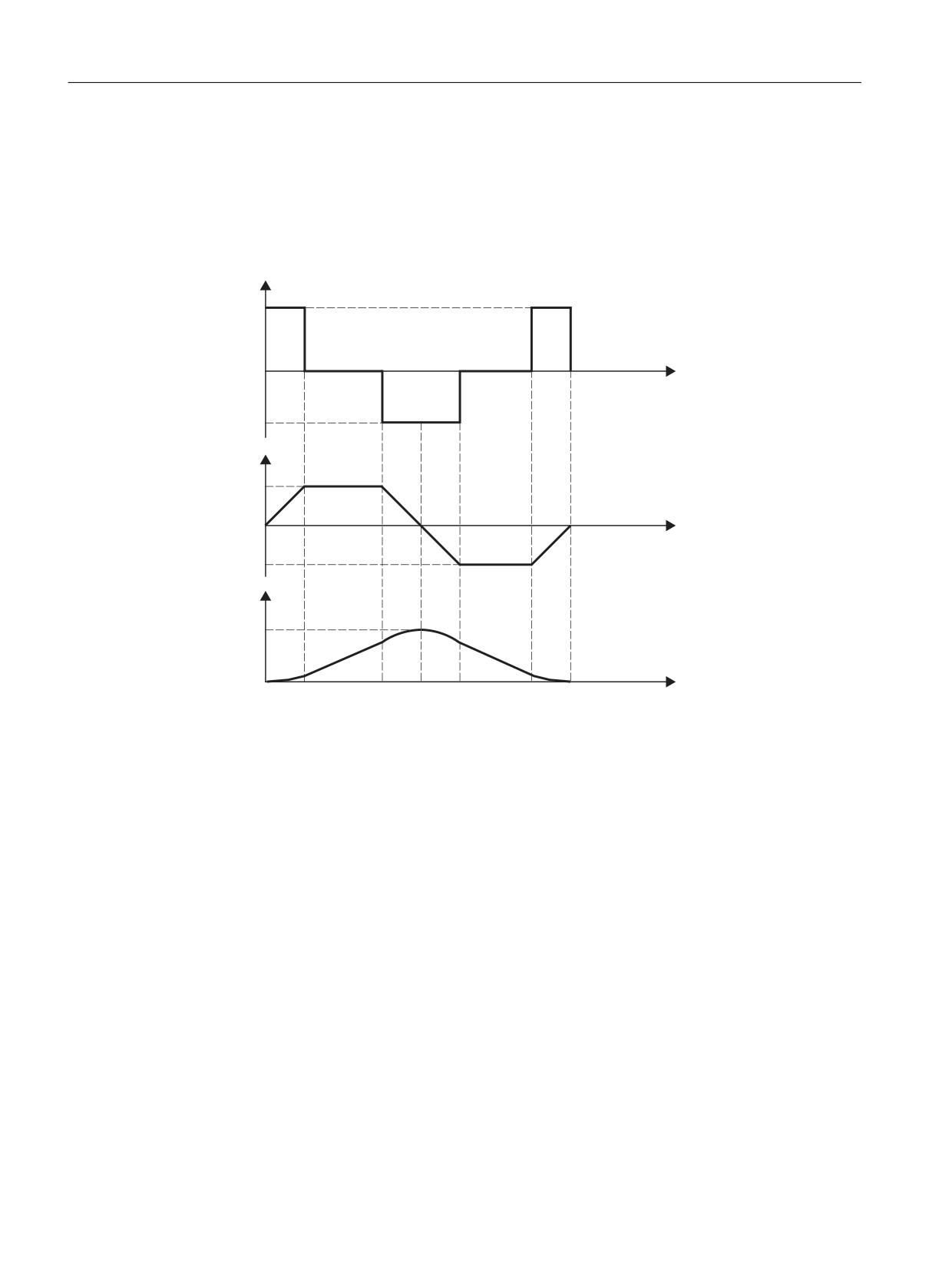
Acceleration profile

U_PD[

D_PD[

Y_PD[

r_max:

Maximum jerk value

a_max:

Maximum acceleration value

v_max:

Maximum velocity value

Time

Figure 4-4

Jerk, acceleration and velocity schematic with jerk limitation acceleration profile

The following features of the acceleration profile can be identified from the figure above:

• Interval: t₀ - t₁

Constant jerk with +r_max; linear increase in acceleration; quadratic increase in velocity

• Interval: t₁ - t₂

Constant acceleration with +a_max; linear increase in velocity

• Interval: t₂ - t₃

Constant jerk with -r_max; linear decrease in acceleration; quadratic decrease in excessive

velocity until maximum value +v_max is reached

• Interval: t₃ - t₄

Constant jerk with +r_max; linear increase in braking acceleration; quadratic decrease in

velocity

Axes and spindles

Function Manual, 10/2020, 6FC5397-4GP40-0BA1

Acceleration and jerk

4.2 Detailed description

• Interval: t

- t₅

Constant braking acceleration with -a_max; linear decrease in velocity

• Interval: t₅ - t₆

Constant jerk with -r_max; linear decrease in braking acceleration; quadratic decrease in

velocity reduction until zero velocity is reached v = 0

4.2.12.2

Parameterization

Maximum jerk value for path motions (axis-specific)

The maximum axial jerk for path motions can be set for the specific technology for each machine

axis via the following machine data:

MD32431 $MA_MAX_AX_JERK[<parameter set index>]

With <parameter set index> = 0, 1, 2 ... (max. parameter set number - 1)

For further information about the technology-specific parameter sets, see the Basic Functions

Function Manual.

The path parameters are calculated by the path planning of the preprocessing so that the

parameterized maximum values of the machine axes involved in the path are not exceeded.

Note

It is possible for the maximum value to be exceeded in connection with specific processing

situations (see Section "Path jerk for real-time events (channel-specific) (Page 101)").

Maximum jerk value for path motions (channel-specific)

In addition to the axis-specific setting, the maximum jerk value can also be specified as channel-

specific path parameter via the following machine data:

MD20600 $MC_MAX_PATH_JERK (path-related maximum jerk)

In order to exclude the mutual influencing of axis and channel-specific maximum jerk values, the

channel-specific maximum value must be set to a value greater than the axial maximum values.

4.2.12.3

Programming

Syntax

SOFT

Functionality

The SOFT part-program instruction is used to select the acceleration profile with jerk limitation

for the traversing operations of geometry axes in the channel.

G group: 21

Axes and spindles

Function Manual, 10/2020, 6FC5397-4GP40-0BA1

Acceleration and jerk

4.2 Detailed description

Effective: Modal

Reset response

The channel-specific initial setting is activated via a reset:

MD20150 $MC_GCODE_RESET_VALUES[20]

Boundary conditions

If the acceleration mode is changed in a part program during machining (BRISK ↔ SOFT), a

block change is performed at the point of transition with an exact stop at the end of the block,

even in continuous-path mode.

4.2.13

Jerk limitation with single-axis interpolation (SOFTA) (axis-specific)

4.2.13.1

Parameterization

Basic setting of axis-specific jerk limitation

Acceleration with jerk limitation can be set as the axis-specific initial setting:

MD32420 $MA_JOG_AND_POS_JERK_ENABLE== TRUE

Maximum axis-specific jerk for positioning axis movements

When traversing positioning axes with active jerk limitation, the value from one of the following

machine data takes effect as the maximum axis-specific jerk:

• MD32430 $MA_JOG_AND_POS_MAX_JERK (maximum axis-specific jerk)

• MD32431 $MA_MAX_AX_JERK [0] (maximum axis-specific jerk for path motions in the

dynamic response mode DYNNORM)

• MD32431 $MA_MAX_AX_JERK [1] (maximum axis-specific jerk for path motions in dynamic

response mode DYNPOS)

The machine data to be used is determined by the set positioning axis dynamic response mode:

MD18960 $MN_POS_DYN_MODE = <mode>

<mode>

Meaning

The following applies as the maximum axis-specific jerk for positioning axis motions:

MD32430 $MA_JOG_AND_POS_MAX_JERK

With active G75 (fixed-point approach): MD32431 $MA_MAX_AX_JERK[ 0 ]

MD32431 $MA_MAX_AX_JERK[ 1 ]

Axes and spindles

Function Manual, 10/2020, 6FC5397-4GP40-0BA1

Acceleration and jerk

4.2 Detailed description

Maximum axial jerk for JOG motions

See Chapter "Acceleration and jerk for JOG motions (Page 123)".

4.2.13.2

Programming

Syntax

SOFTA (Axis {Axis})

Functionality

The SOFTA part-program command is used to select acceleration with jerk limitation for single-

axis movements (positioning axis, reciprocating axis, etc.)

G group: -

Effectiveness: Modal

Axis:

• Value range: Axis name of the channel axes

Axis-specific initial setting

Acceleration with jerk limitation can be set as the axis-specific initial setting for single-axis

movements:

MD32420 $MA_JOG_AND_POS_JERK_ENABLE = TRUE

Reset behavior

The axis-specific initial setting is activated via a reset:

MD32420 $MA_JOG_AND_POS_ENABLE

4.2.14

Limiting the path jerking (channel-specific)

4.2.14.1

Function

To be able to flexibly respond to the respective preprocessing situation, the path jerk calculated

by preprocessing can be channel-specifically limited via setting data:

SD42510 $SC_SD_MAX_PATH_JERK (maximum path jerk)

The value specified in the setting data is only taken into consideration if it is smaller than the path

jerk calculated by preprocessing.

The limitation must be enabled channel-specifically via setting data:

SD42512 $SC_IS_SD_MAX_PATH_JERK = TRUE

Axes and spindles

Function Manual, 10/2020, 6FC5397-4GP40-0BA1

Acceleration and jerk

4.2 Detailed description

4.2.14.2

Parameterization

Parameterization is carried out for specific channels using setting data:

SD42510 $SC_SD_MAX_PATH_JERK (maximum path jerk)

SD42512 $SC_IS_SD_MAX_PATH_JERK

(activation of path-jerk limitation)

4.2.14.3

Programming

Maximum path jerk

Syntax

$SC_SD_MAX_PATH_JERK = jerk value

Functionality

The path-jerk limitation can be adjusted for the situation by programming the setting data.

Jerk value:

• Value range: ≥ 0

• Unit: m/s³

Application:

• Part program

• Static synchronized action

Switch ON/OFF

Syntax

$SC_IS_SD_MAX_PATH_JERK = value

Functionality

The path-jerk limitation can be activated/deactivated by programming the setting data.

Parameter: Value

• Value range: TRUE, FALSE

Axes and spindles

100

Function Manual, 10/2020, 6FC5397-4GP40-0BA1

Acceleration and jerk

4.2 Detailed description

Application:

• Part program

• Static synchronized action

4.2.15

Path jerk for real-time events (channel-specific)

4.2.15.1

Function

So that no compromise has to be made between machining-optimized jerk on the one hand and

time-optimized jerk in connection with the following real-time events on the other:

• NC Stop / NC Start

• Changing the feedrate override

• Changing the velocity default for "safely reduced velocity" within the context of the "Safety

Integrated" function

for the real-time events mentioned, the path jerk can be specified using a channel-specific

system variable:

$AC_PATHJERK = path jerk

Path jerk for real-time events will only be active for the duration of the change in velocity in

respect of one of the real-time events specified above.

Limitation

As the jerk is not a physical variable of any relevance to the drive, no limit is imposed on the jerk

set.

Effectiveness

Effective

Path jerk for real-time events is only enabled in AUTOMATIC and MDA operating modes

in conjunction with the following real-time events:

• NC Stop / NC Start

• Override changes

• Changing the velocity default for "safely reduced velocity" within the context of the

"Safety Integrated" function

Not effective

Path jerk for real-time events is ineffective for changes in the path velocity that are

attributable to path planning during preprocessing for the channel, such as contour

curvatures, corners, kinematic transformation limitations, etc.

Path jerk for real-time events is ineffective if the programmed value is smaller than the

path jerk calculated during preprocessing for the path section concerned.

Axes and spindles

Function Manual, 10/2020, 6FC5397-4GP40-0BA1

101

Acceleration and jerk

4.2 Detailed description

Programming

For the purpose of setting the jerk for real-time events in accordance with the acceleration, the

system variables can be set as follows:

$AC_PATHJERK = $AC_PATHACC/smoothing time

• $AC_PATHACC: Path acceleration [m/s²]

Smoothing time: Freely selectable, e.g. 0.02 s

For information about programming system variables in the part program or synchronized

actions, see Section "Programming (Page 102)".

4.2.15.2

Programming

Syntax

$AC_PATHJERK = path jerk

Functionality

The path jerk for real-time events is set via the channel-specific system variables.

Jerk value:

• Value range: Path jerk ≥ 0

• Unit: m/s³

Application:

• Part program

• Static synchronized action

Reset behavior

The function is deactivated on reset.

Boundary conditions

Programming $AC_PATHJERK in the part program automatically triggers a preprocessing stop

with REORG (STOPRE).

4.2.16

Jerk during programmed rapid traverse (G00) (axis-specific)

4.2.16.1

Function

Frequently the maximum jerk for the machine axes participating in processing must be set lower

than that which corresponds to the performance capability of the machine, due to the

processing-specific constraints.

Axes and spindles

102

Function Manual, 10/2020, 6FC5397-4GP40-0BA1

Acceleration and jerk

4.2 Detailed description

For time-optimized traversing of the machine axes for programmed rapid traverse (part program

instruction G00), a separate maximum value of the axis-specific jerk can be parameterized.

JOG setup mode

The jerk during rapid traverse override (ROV) in JOG setup mode is not affected by this

functionality.

4.2.16.2

Parameterization

The maximum value for axis-specific jerk with programmed rapid traverse is parameterized

(G00) using the axis-specific machine data:

MD32434 $MA_G00_ACCEL_FACTOR

(scaling of the acceleration limitation with G00)

This is used to generate the maximum value for axis-specific jerk with programmed rapid

traverse (G00) that is taken into account by the path planning component during preprocessing:

Jerk[axis] =

MD32431 $MA_MAX_AX_JERK * MD32435 $MA_G00_JERK_FACTOR

4.2.17

Excessive jerk for block transitions without constant curvature (axis-specific)

4.2.17.1

Function

In the case of block transitions without constant curvature (e.g. straight line > circle), the

programmable controller has to decelerate movement of the geometry axes significantly in

order to ensure compliance with the parameterized axis dynamics. To reduce or prevent the

deceleration at block transitions without constant curvature, a higher axis-specific jerk can be

allowed.

The increase in jerk is parameterized via a separate axis-specific maximum value.

4.2.17.2

Parameterization

The excessive jerk for block transitions without constant curvature is parameterized using the

axis-specific machine data:

MD32432 $MA_PATH_TRANS_JERK_LIM

(excessive jerk for block transitions without constant curvature)

Axes and spindles

Function Manual, 10/2020, 6FC5397-4GP40-0BA1

103

Acceleration and jerk

4.2 Detailed description

4.2.18

Velocity-dependent jerk adaptation (axis-specific)

Function

The dynamic path response results from the parameterized, constant axial maximum values for

velocity, acceleration and jerk of the axes involved in the path:

• MD32000 $MA_MAX_AX_VELO (maximum axis velocity)

• MD32300 $MA_MAX_AX_ACCEL (maximum axis acceleration)

• MD32431 $MA_MAX_AX_JERK (max. axial jerk for path motion)

For contours with non-constant curvature (torsion), as for example in connection with free-

form surfaces, fluctuations in the path velocity, particularly in the upper velocity range, can

result mainly due to the axial jerk. The fluctuations of the path velocity lead to adverse affects in

the surface quality.

The influence of the axial jerk on the path velocity is decreased for contours with non-constant

curvature through a velocity-dependent increase of the permissible axial jerk. Fluctuations in

the path velocity can be avoided with the appropriate parameterization.

The velocity-dependent increase of the permissible axial jerk has no effect on the maximum

possible path acceleration and path jerk. These result from the constant axial maximum values

parameterized in the in the machine data even when jerk adaptation is active.

As both curvature and torsion are zero in the case of linear motion, the velocity-dependent jerk

adaptation has no effect with linear motions.

Availability

The "velocity-dependent jerk adaptation" function is available independent of the function

"Freeform surface mode: Basic functions".

For further information about the function "Freeform surface mode: Basic functions" refer to

the Basic Functions Function Manual.

Axes and spindles

104

Function Manual, 10/2020, 6FC5397-4GP40-0BA1

Acceleration and jerk

4.2 Detailed description

Parameter assignment

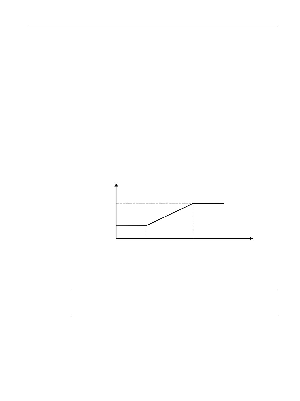
The "Velocity-dependent jerk adaptation" function is parameterized with the following machine

data:

• MD32437 $MA_AX_JERK_VEL0[<n>] = <threshold value_lower>

Lower velocity threshold of the jerk adaptation. Velocity-dependent jerk adaptation takes

effective as of this velocity.

The lower velocity threshold can be set separately via index n for each dynamic response

mode.

• MD32438 $MA_AX_JERK_VEL1[<n>] = <threshold value_upper>

Upper velocity threshold of the jerk adaptation. The velocity-dependent jerk reaches its

maximum value j_max parameterized with MD32439 $MA_MAX_AX_JERK_FACTOR at this

velocity.

The upper velocity threshold can be set separately via index n for each dynamic response

mode.

• MD32439 $MA_MAX_AX_JERK_FACTOR = <factor>

Factor for the parameterization of the maximum velocity-dependent jerk j_max on reaching the

upper velocity threshold MD32438 $MA_AX_JERK_VEL1[<n>]:

j_max = (MD32431 $MA_MAX_AX_JERK) * (MD32439 $MA_MAX_AX_JERK_FACTOR)

The velocity-dependent jerk adaptation is active at a value > 1.0.

The velocity-dependent jerk adaptation is inactive at a value = 1.0.

PD[LPXP SHUPLWWHG

D[LDO MHUN

$[LV VSHHG

v₀:

MD32437 $MA_AX_JERK_VEL0

v₁:

MD32438 $MA_AX_JERK_VEL1

j₀:

MD32431 $MA_MAX_AX_JERK

j₁:

MD32439 $MA_MAX_AX_JERK_FACTOR * MD32431 $MA_MAX_AX_JERK

Figure 4-5

Axial jerk as a function of the axis velocity

Note

The velocity-dependent jerk adaptation is only active, if:

MD32439 $MA_MAX_AX_JERK_FACTOR > 1.0

Axes and spindles

Function Manual, 10/2020, 6FC5397-4GP40-0BA1

105

Acceleration and jerk

4.2 Detailed description

Example

Example of parameter assignment:

• MD32437 $MA_AX_JERK_VEL0 = 3000 mm/min

• MD32438 $MA_AX_JERK_VEL1 = 6000 mm/min

• MD32439 $MA_MAX_AX_JERK_FACTOR[AX1] = 2.0

• MD32439 $MA_MAX_AX_JERK_FACTOR[AX2] = 3.0

• MD32439 $MA_MAX_AX_JERK_FACTOR[AX3] = 1.0

Effect

• The speed-dependent jerk adaptation is active for the 1st and 2nd axis, whereas the function

for the 3rd axis is not active.

• The parameterized jerk is effective at axis velocities in the range of 0 to 3000 mm/min.

• The maximum jerk is linearly increased for axis velocities in the range 3000 mm/min to

6000 mm/min.

• The maximum permitted jerk of the 1st axis is, for axis velocities greater than 6000 mm/min,

increased by a factor of 2 - for the 2nd axis, by factor of 3.

• The parameterized values apply in each dynamic response mode.

4.2.19

Jerk filter (position setpoint filter, axis-specific)

4.2.19.1

Function

In certain application scenarios, e.g. when milling free-form surfaces, it may be beneficial to

smooth the position setpoint characteristics of the machine axes. This enables the surface

quality to be improved by reducing the mechanical vibration generated in the machine.

To smooth the position setpoint characteristic of a machine axis, a jerk filter can be activated at

the position controller level, independent of channel- and axis-specific jerk limitations that are

taken into account at interpolator level. Jerk limitation can be set using the following machine

data, for example:

• MD20600 $MA_MAX_PATH_JERK (pathrelated maximum jerk)

• MD32431 $MA_MAX_AX_JERK (maximum axial jerk for path motion)

All position setpoint filter types have a lowpass characteristic, and always round a contour at the

center of the curvature (towards the inside). Larger time constants or lower filter frequencies

round the contour more significantly; however, that also means that machine resonance points

(machine oscillation) are excited less. A compromise must always be found between an

adequate damping effect and contour accuracy.

The damping effect can be monitored via the positioning response, the contour accuracy using

a circularity test, for example.

Axes and spindles

106

Function Manual, 10/2020, 6FC5397-4GP40-0BA1

Acceleration and jerk

4.2 Detailed description

Various filter types are available to enable the jerk filter to be optimally matched to the specific

machine characteristics:

• 2nd order filter (PT2)

• Moving average calculation

• Bandstop

• Double sliding averaging

• FIR lowpass (FIR: Finite Impulse Response)

Filter type: 2nd order filter

Because it is a simple lowpass filter, a filter type "2nd order filter" can only meet the requirements

specified above where relatively small filter time constants (around 10 ms) are involved. When

used in conjunction with larger time constants, inadmissible contour deviations soon become

apparent. The filter effect is relatively low.

This filter type is the default for historical reasons.

Filter type: Moving average calculation

Where low contour deviations are required, filter time constants within the range of 20 - 40 ms

can be set using the "moving averaging" filter type. The smoothing effect is largely symmetrical.

The display of the calculated servo gain factor (K_V) in the user interface, indicates smaller values

than would normally be appropriate for the filter. The contour accuracy is higher than the

displayed servo gain factor (K_V) appears to suggest.

When changing from "2nd order filter" to "sliding averaging" filter type, the displayed servo gain

factor (K_V) may therefore decrease (with identical filter time constant), even though there is an

improvement in contour accuracy.

Filter type: Bandstop

The use is not recommended and is (still) only available for compatibility reasons.

The band-stop filter is a 2nd order filter in terms of numerator and denominator:

V '=

˭ I

V '1

˭ I1

With:

f_N:

Numerator natural frequency

f_D:

Denominator natural frequency

D_N:

Numerator damping

D_D:

Denominator damping

Axes and spindles

Function Manual, 10/2020, 6FC5397-4GP40-0BA1

107

Acceleration and jerk

4.2 Detailed description

Since a vibration-capable filter setting is not expected to yield useful results in any case, as with

the "2nd-order filter" (PT2) low-pass filter (PT2) type of the jerk filter there is no setting option for

the denominator damping D_D. The denominator damping D_D is permanently set to 1.

The band-stop filter can be parameterized in two different ways:

• Real band-stop filter

• Band-stop filter with additional amplitude response increase/decrease at high frequencies

Real band-stop filter

A real band-stop filter is obtained when identical numerator and denominator natural

frequencies are selected:

f_N = f_D = f_block (blocking frequency)

If the numerator damping setting = 0 is selected, the blocking frequency is equivalent to

complete attenuation. In this case the 3 dB bandwidth is calculated as follows:

f_{3 dB bandwidth} = 2 * f_block

If instead of complete attenuation, a reduction by a factor of k is all that is required, then

numerator damping should be selected in accordance with k. In this case the above formula for

calculating the 3 dB bandwidth no longer applies.

Band-stop filter with additional amplitude response increase/decrease at high frequencies

In this case, the numerator and denominator natural frequencies are set to different values. The

numerator natural frequency determines the blocking frequency.

By selecting a lower/higher denominator natural frequency than the numerator natural

frequency, you can increase/decrease the amplitude response at high frequencies. An amplitude

response increase at high frequencies can be justified in most cases, as the controlled system

generally has a lowpass characteristic itself, i.e. the amplitude response decreases at high

frequencies anyway.

Constraints

If the numerator natural frequency is selected to be too high, then the filter is deactivated. In this

case, the frequency limit f_Zmax depends on the position controller clock cycle:

6KDQQRQ 7KHRUHP

I=PD[

3RVLWLRQ FRQWURO F\FOH FORFN

=PLQ

Filter type: Double sliding averaging

Double moving average calculation has a stronger smoothing effect than basic moving average

calculation. By additionally parameterizing a second moving average calculation, differences in

the dynamic response between axes that are interpolating with one another can be

compensated.

Axes and spindles

108

Function Manual, 10/2020, 6FC5397-4GP40-0BA1

Acceleration and jerk

4.2 Detailed description

Filter type: FIR lowpass

Note

To use the jerk filter type "FIR lowpass", a license is required for the following option:

"Top Speed" (article number: 6FC5800-0AS13-0Yx0)

Note

The use of the "FIR lowpass" type of jerk filter is only permitted with active jerk limitation (SOFT/

SOFTA).

Using a FIR lowpass as jerk filter allows the required smoothing effect to be specified in the

frequency range. Normally, a FIR lowpass filter has a more significant damping effect with

improved contour accuracy than all of the previously described jerk filter types.

FIR lowpass dynamic response-dependent

The filter settings can be made separately for each dynamic mode (DYNNORM, DYNPOS,

DYNROUGH, DYNSEMIFIN, DYNFINISH, DYNPREC) for the dynamic-dependent FIR lowpass jerk

filter variant, independently of the use in filter circuit 1 or 2 (Page 177). Thus, it is possible to set

the effective damping and the resulting overshot behavior to the processing type or the

expected workpiece quality.

When the CALCFIR (Page 112) NC language command is executed in the "CUST_832"

manufacturer cycle, the dynamic response-dependent FIR jerk filter settings for the active

dynamic response mode in all axes of a channel with active FIR filters are matched to the dynamic

response-limiting linear axis and made effective, thus ensuring path interpolation for all channel

axes involved.

When the control system powers up, for a channel reset and end of program reset, the FIR jerk

filter settings are automatically activated to match the initial setting of G group 59.

Example:

If it is important to have a minimal processing time for DYNROUGH and the highest processing

accuracy and surface quality for DYNFINISH or DYNPREC, these requirements can be fulfilled

using two different FIR jerk filter settings. The NC language command CALCFIR adapts the FIR jerk

filter to the programmed dynamic mode for all of the axes of a channel with active FIR filters and

ensures an identical damping effect and contour accuracy.

4.2.19.2

Parameterization

Activation

The jerk filter is activated using the machine data:

MD32400 $MA_AX_JERK_ENABLE (axial jerk limitation)

The jerk filter is active in all operating modes and with all types of interpolation.

Axes and spindles

Function Manual, 10/2020, 6FC5397-4GP40-0BA1

109

Acceleration and jerk

4.2 Detailed description

Filter type

The filter type is selected via the machine data:

MD32402 $MA_AX_JERK_MODE (filter type for axial jerk limitation)

Value

Filter type

2nd order filter

Moving average calculation

Bandstop

Double sliding averaging

FIR lowpass

Axial jerk filters (filter types 1, 2 and 3)

The axial jerk filters are set using the following machine data:

• For filter types 1 and 2 with MD32410 $MA_AX_JERK_TIME.

• For filter type 3 using machine data MD32412 AX_JERK_FREQ and MD 32414

AX_JERK_DAMP.

The jerk filter is only effective when the time constant is greater than a position control clock

cycle.

Double sliding averaging (filter type 4)

A double moving average calculation requires that the following machine data are set:

• MD32410 $MA_AX_JERK_TIME

• MD32411 $MA_AX_JERK_TIME_ADD

If both machine data are parameterized the same, a delta filter is implemented, which produces

extremely strong damping, but also significant contour distortion.

FIR lowpass (filter type 5)

A FIR lowpass filter requires that the following machine data are set:

• MD32407 $MA_AX_JERK_FIR_FREQ = (corner frequency (-6dB) of the axial FIR jerk filter

smoothing)

• MD32408 $MA_AX_JERK_FIR_ORDER (order of the filter for the axial FIR jerk filter smoothing)

• MD32409 $MA_AX_JERK_FIR_ORDER (window type of the axial FIR jerk filter smoothing):

- Window type 0 does not use a window.

- Window type 1 uses a Hamming window.

- Window type 2 uses a Blackman-Harris window.

- Window type 3 uses a Gauss window.

Axes and spindles

110

Function Manual, 10/2020, 6FC5397-4GP40-0BA1

Acceleration and jerk

4.2 Detailed description

FIR lowpass dynamic response-dependent (filter type 5)

A dynamic response-dependent FIR lowpass requires that the following machine data be set:

• MD32404 $MA_CALCFIR_SELECT (FIR lowpass - activation of the dynamic response-

dependent filter circuit)

Value

Meaning

CALCFIR calculation is inactive for this axis

CALCFIR calculation effects the 1st filter circuit

CALCFIR calculation effects the 2nd filter circuit

• MD32405 $MA_CALCFIR_FREQ[<n>] (FIR lowpass - frequency [Hz])

• MD32406 $MA_CALCFIR_TOL[<n>] (FIR lowpass - tolerance [mm])

• MD32431 $MA_MAX_AX_JERK[<n>] (maximum axial jerk for path movement)

<n>: Dynamic response mode (0 = DYNNORM, 1 = DYNPOS, 2 = DYNROUGH, 3 = DYNSEMIFIN,

4 = DYNFINISH, 5 = DYNPREC)

The FIR lowpass frequency must usually be selected somewhat above or on the mechanical

natural frequency of the axis. With the FIR lowpass tolerance, the maximum permissible

overshot of the filter is defined during a positioning action (does not correspond to the contour

accuracy). The higher the selected permissible FIR lowpass tolerance, the more accurately the

filter for curvature changes becomes; the contour accuracy of the workpiece is increased. The

maximum permissible overshot of the filter in MD32406 $MA_CALCFIR_TOL is only adhered to

up to a jerk of MD32431 $MA_MAX_AX_JERK. If the jerk is adapted above this value with the aid

of the "Intelligent Load Control" (Page 979) function, higher overshoot may occur.

Example:

• Tolerance = 0.003 [mm]

• Frequency = 25 [Hz]

The CALCFIR (Page 112) NC language command adapts the dynamic-dependent FIR jerk filters

in all axes of a channel with active FIR filters to the dynamic response-limiting linear axis.

The following FIR lowpass machine data are written:

• MD32407 $MA_AX_JERK_FIR_FREQ (corner frequency of the axial FIR jerk filter smoothing)

• MD32408 $MA_AX_JERK_FIR_ORDER (order of the filter for the axial FIR jerk filter smoothing)

Programmable contour accuracy

With heavily damping filters with low filter frequency, the contour accuracy in curvatures can be

adhered to through the use of the "Programmable contour accuracy" function.

If the function is used in combination with the jerk filter type "FIR lowpass", the setting of the

following machine data is required:

MD38020 $MA_MM_CPREC_FIR_POINTS (number of points for characteristic approximation of

FIR filters for CPRECON)

Recommended setting = 100

For further information on the topic "Programmable contour accuracy", see Monitoring and

Compensating Function Manual.

Axes and spindles

Function Manual, 10/2020, 6FC5397-4GP40-0BA1

111

Acceleration and jerk

4.2 Detailed description

4.2.19.3

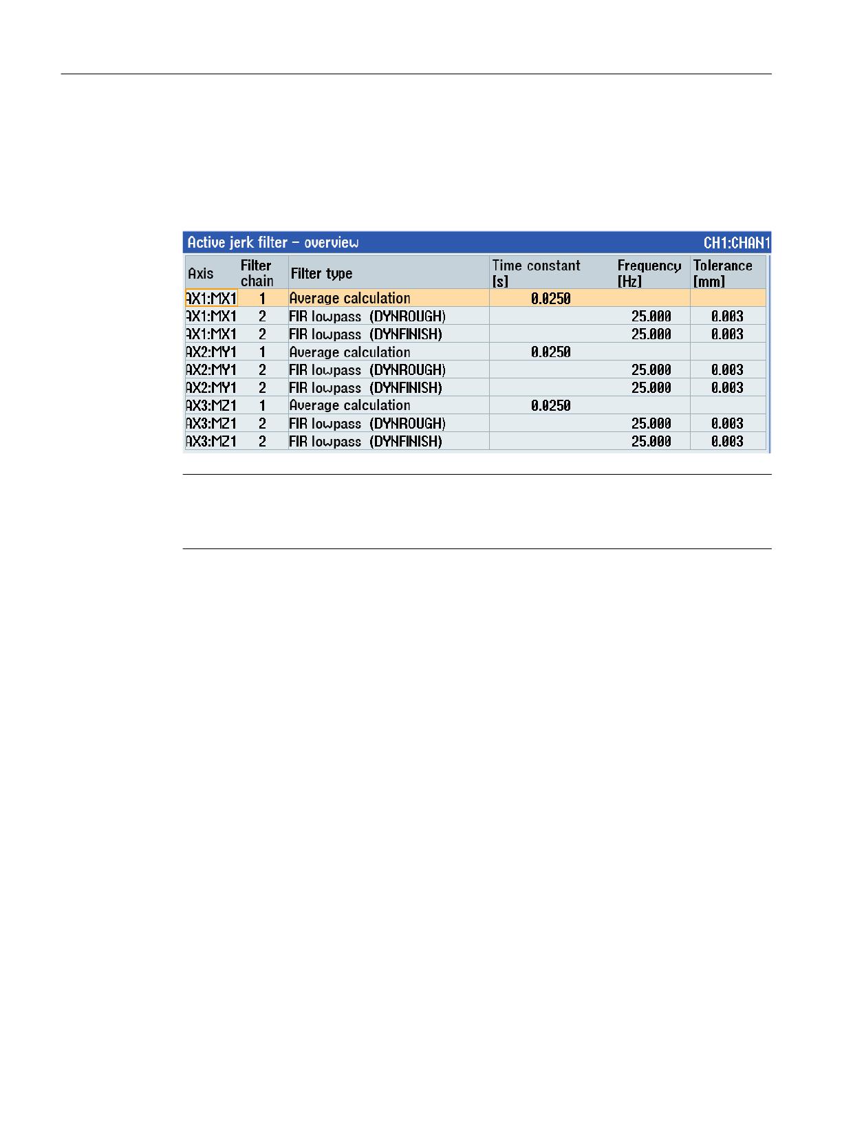
Active jerk filters - overview

All of the active jerk filters in the channel are displayed in tabular format in the operator interface

(SINUMERIK Operate, "Setup" operating area > "NC" > "Jerk filter").

Example:

Note

A jerk filter is active and displayed if the following is true:

MD32400 $MA_AX_JERK_ENABLE = 1

4.2.19.4

Programming

In order to achieve an identical damping effect and contour accuracy for all axes in the channel

for which an FIR low-pass jerk filter is active after changing the dynamic mode, the dynamic

response-dependent FIR filter settings can be calculated and made effective with the NC voice

command CALCFIR.

Application

CALCFIR is used in the CUST_832 manufacturer cycle.

Standard workflow

CYCLE832 is programmed at the start of an NC program for free-form surface machining. When

the program is being executed, CYCLE832 calls the manufacturer cycle CUST_832 and the NC

language command CALCFIR inserted by the machine manufacturer in CUST_832 is executed.

Effectiveness

The filter settings overwritten by CALCFIR remain active until they are again overwritten by the

next CALCFIR call. This is always required, if, using a command of G group 59 (dynamic response

mode for path interpolation), a change to the actual dynamic response mode is programmed.

Response when the control system powers up / channel reset / end of program reset

When the control system powers up, and for a channel/end of program reset, the FIR filter

settings are activated to match the initial setting of G group 59.

Axes and spindles

112

Function Manual, 10/2020, 6FC5397-4GP40-0BA1

Acceleration and jerk

4.2 Detailed description

Requirements

• Option "Top Speed" is set.

Note

To achieve optimum results with "Top Speed", it is recommended that option "Top Surface"

is also used.

• The following conditions must be satisfied for axes in the interpolation group:

- FIR low-pass jerk filter is active.

- FIR filter settings dependent on the dynamic response are configured.

- Overwriting filter settings by CALCFIR is enabled.

• Jerk limiting SOFT/SOFTA is active.

Syntax

CALCFIR is programmed in a separate block. The call in the manufacturer cycle CUST_832 is

realized directly after programming the dynamic response mode:

DYN...

CALCFIR

Meaning

DYN...:

Command from G group 59 to select the dynamic response mode

DYNNORM:

Activate normal dynamic response

DYNPOS:

Activate dynamic response for positioning mode, tapping

DYNROUGH:

Activate dynamic response for roughing

DYNSEMIFIN:

Activate dynamic response for semi-finishing

DYNFINISH:

Activate dynamic response for finishing

DYNPREC:

Activate dynamic response for smooth-finishing

CALCFIR:

Predefined procedure to dynamically adapt the FIR low-pass jerk filters

Note

CALCFIR performs an implicit NEWCONFIG to activate the result of the FIR filter calculation - both

in the axis-specific machine data to parameterize the FIR low-pass jerk filter as well as for

CPRECON. The implicit NEWCONFIG means that additional NEWCONFIG-relevant machine data

become active.

Axes and spindles

Function Manual, 10/2020, 6FC5397-4GP40-0BA1

113

Acceleration and jerk

4.2 Detailed description

Boundary conditions

Use in synchronized actions

CALCFIR cannot be programmed in synchronized actions.

4.2.20

Knee-shaped acceleration characteristic

4.2.20.1

Function: Adaptation to the motor characteristic curve

Various motor types, particularly stepper motors, have a torque characteristic that is highly

dependent on the speed with a steep decline in the torque in the upper speed range. For optimal

utilization of the motor characteristic, the acceleration of the associated NC axis must be

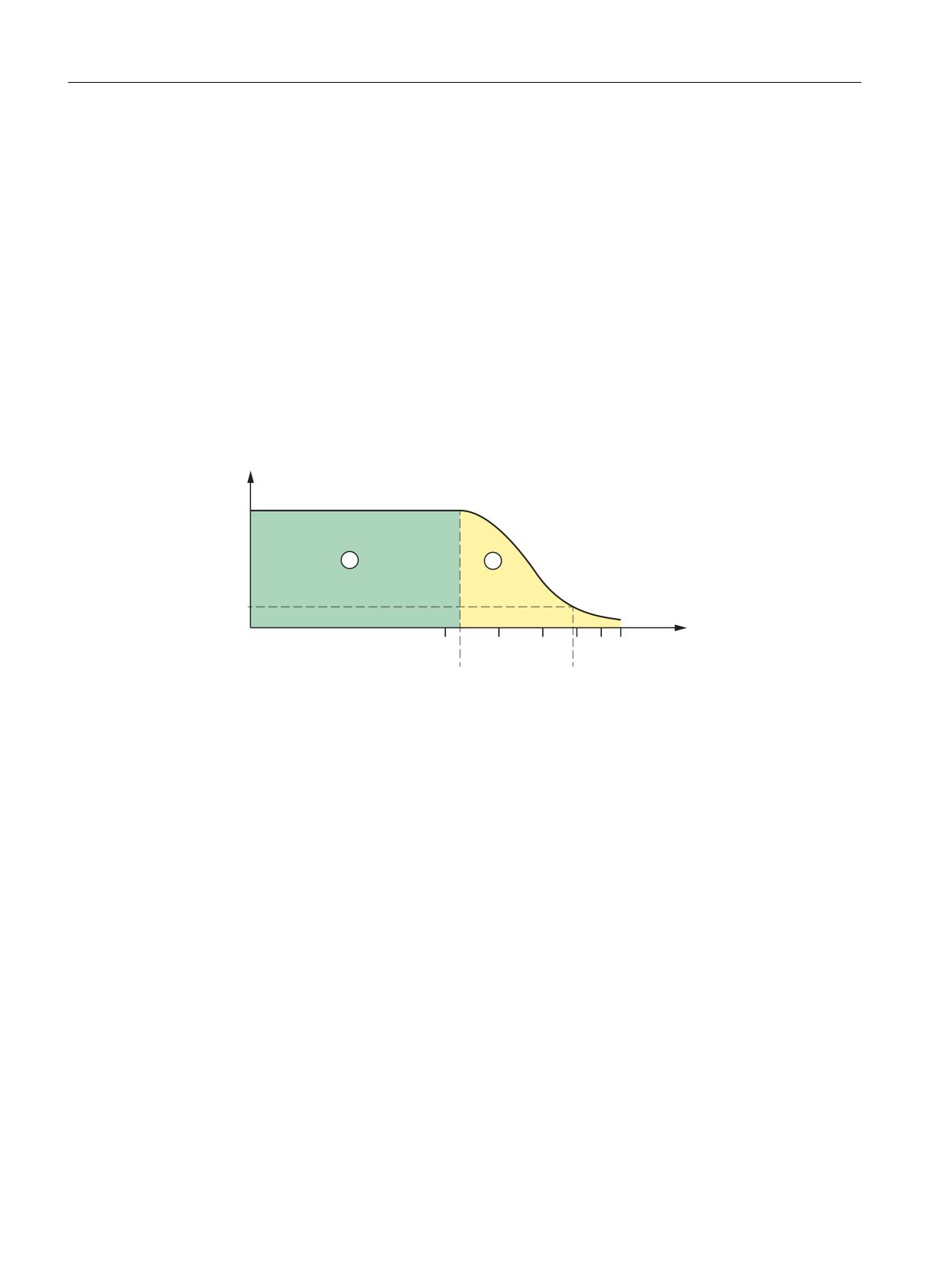
reduced as of a specific speed.

0 >1P@

0_PD[

0_UHG

Q_UHG

Q_PD[

① Normal range

② Reducing range

n_red

Speed as of which traversing is done with reduced torque

n_max

Maximum speed

M_max

Maximum torque

M_red

Torque at n_max (corresponds to acceleration reduction)

Characteristic curve types

As a controller-internal emulation of the torque characteristic curve of the motor, the following

characteristic curve types can be selected for the reducing range (see chapter "Parameterization

(Page 118)"):

• Constant torque characteristic

• Hyperbolic torque characteristic

• Linear torque characteristic

Axes and spindles

114

Function Manual, 10/2020, 6FC5397-4GP40-0BA1

Acceleration and jerk

4.2 Detailed description

4.2.20.2

Function: Effects on the path acceleration

The path acceleration characteristic curve results from the types of characteristic curve for the

axes that are of relevance for the path. If axes with different types of characteristic curve are

interpolated together, the acceleration profile for the path acceleration will be determined on

the basis of the reduction type that is most restrictive.

The following order of priorities applies, whereby 1 = top priority:

1. Acceleration reduction: 0 = constant characteristic

2. Acceleration reduction: 1 = hyperbolic characteristic

3. Acceleration reduction: 2 = linear characteristic

4. No acceleration reduction effective

A situation where no acceleration reduction is active arises for example when:

MD35220 $MA_ACCEL_REDUCTION_SPEED_POINT = 1

and / or

MD35230 $MA_ACCEL_REDUCTION_FACTOR = 0

Note

Machine axes featuring stepper motor and DC drive can be interpolated together.

4.2.20.3

Function: Substitute curve

If the programmed path cannot be traversed with the acceleration curve parameterized in the

machine data of the participating axes, e.g. if kinematic transformation and acceleration

types BRISK or SOFT are active, a substitute curve is generated by reducing the dynamic limit

values. The reduced dynamic limit values are calculated to ensure that the substitute

characteristic curve provides the best possible compromise between maximum velocity and

constant acceleration.

Axes and spindles

Function Manual, 10/2020, 6FC5397-4GP40-0BA1

115

Acceleration and jerk

4.2 Detailed description

Substitute characteristic curve with linear path sections

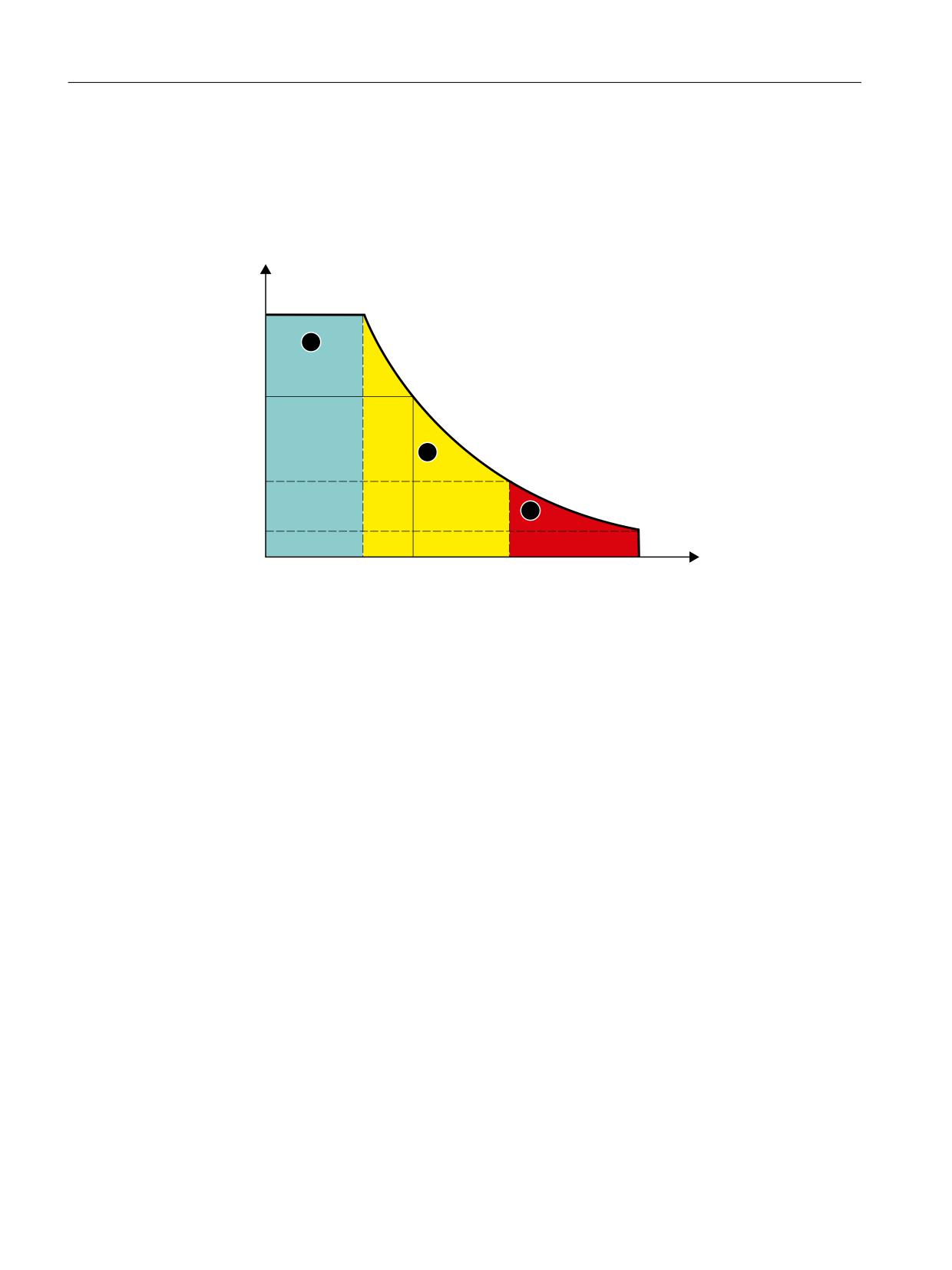
Limitation to this value is applied if the programmed path velocity is greater than that at which

15 % of the maximum acceleration capacity is still available (v_15%a). Consequently, 15 % of the

maximum acceleration capacity/motor torque always remains available, whatever the

machining situation.

D_PD[

D_HUV

D_UHG

Y_UHG

Y_SURJ

Y_PD[

① Normal range

② Reducing range

③ Locked area

a_ers:

Substitute characteristic curve constant acceleration

a_15%

Minimal constant acceleration

a_15% = 0.15 * (a_max- a_red) + a_red

v_ers

Substitute characteristic curve velocity

v_prog

Programmed velocity

v_15%a

Velocity at a_15%

Figure 4-6

Substitute path characteristic curve: Linear path

Axes and spindles

116

Function Manual, 10/2020, 6FC5397-4GP40-0BA1

Acceleration and jerk

4.2 Detailed description

Substitute characteristic curve with curved path sections

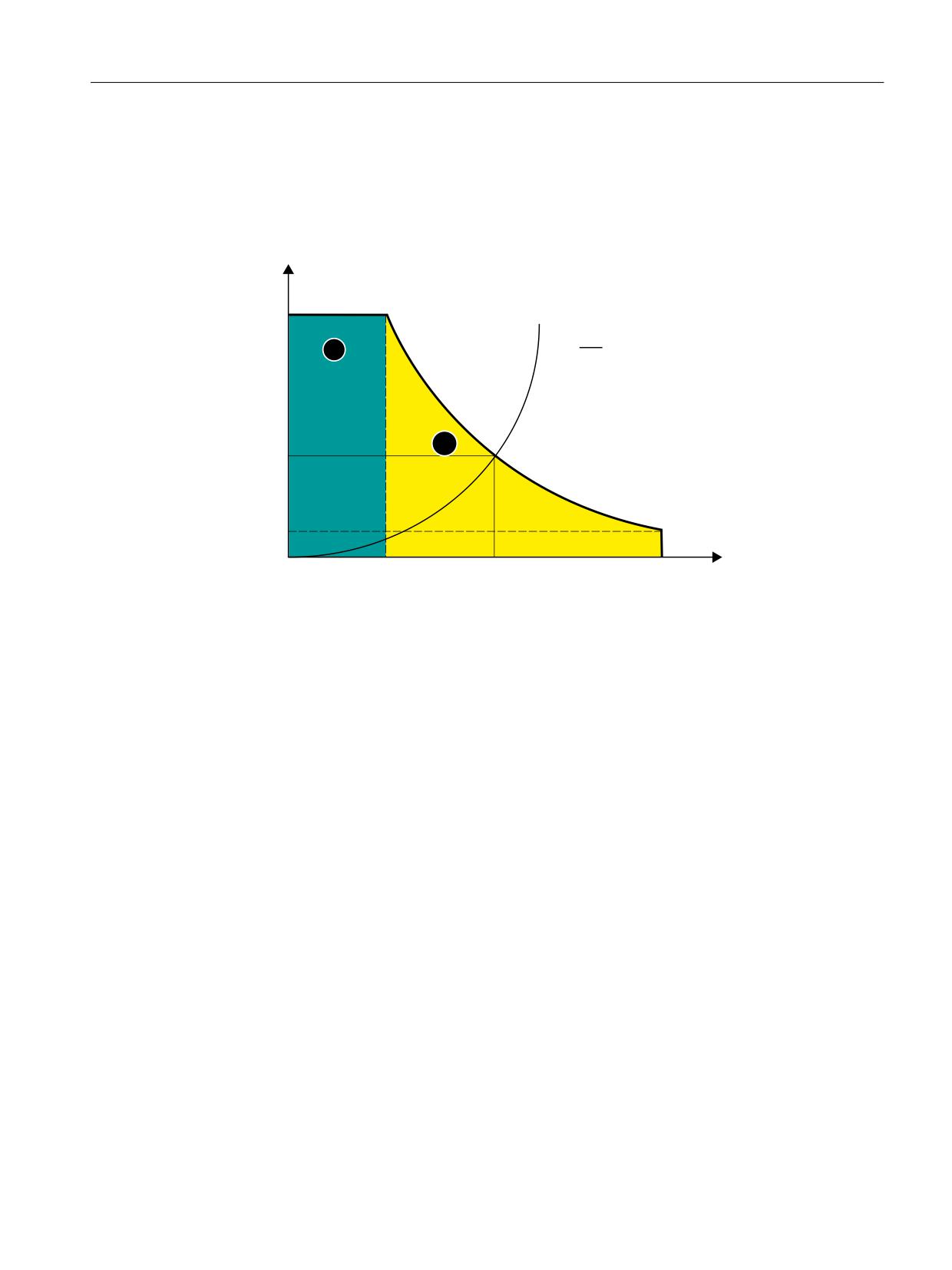
In the case of curved path sections, normal and tangential acceleration are considered together.

The path velocity is reduced so that only up to 25 % of the speed-dependent acceleration

capacity of the axes is required for normal acceleration. The remaining 75 % of the acceleration

capacity is set aside for the tangential acceleration, i.e., deceleration/acceleration on the path.

D_PD[

D₁

D_HUV

D_UHG

Y_UHG

Y_HUV

Y_PD[

① Normal range

② Reducing range

a_N

Normal acceleration

a_ers:

Substitute characteristic curve constant acceleration

v_ers

Substitute characteristic curve velocity

Path radius

Figure 4-7

Substitute path characteristic curve: Curved path

Block transitions with continuous-path mode

If continuous-path mode is active, non-tangential block transitions result in axial velocity jumps

when the programmed path velocity is used for traversing.

As a result, the path velocity is controlled in such a way that prevents any axial velocity

proportion from exceeding the creep velocity v_red at the time of the block transition.

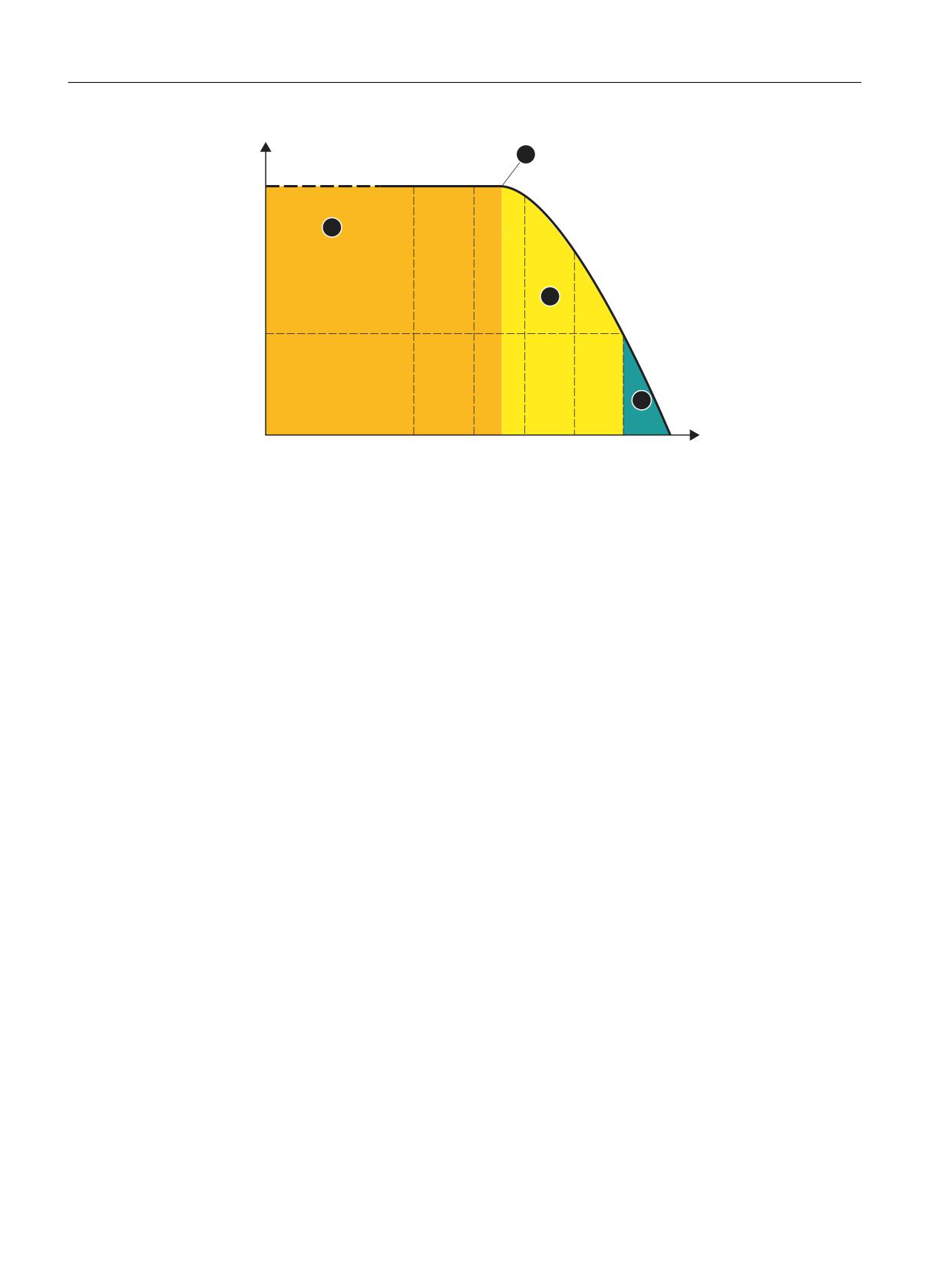
Deceleration ramp with continuous-path mode and LookAhead

In the case of consecutive traversing blocks with short paths, an acceleration or deceleration

operation may be spread over several part program blocks.

In such a situation the "LookAhead" function also takes into account the parameterized speed-

dependent acceleration characteristic.

Axes and spindles

Function Manual, 10/2020, 6FC5397-4GP40-0BA1

117

Acceleration and jerk

4.2 Detailed description

D_PD[

D_HUV

D_UHG

① Normal range ⇒ a = a_max

② Reducing range ⇒ a < a_max

③ Constant travel range ⇒ a = 0 m/s²

④ Brake application point

v_red:

Creep velocity

v_max

Maximum velocity

Traversing block with block number Nx

Figure 4-8

Deceleration with LookAhead

4.2.20.4

Parameterization

Path axis

Parameter assignment

The parameterization of the axis-specific velocity limit, above which the reduced acceleration

acts as an axis for traversing movements, is done via the machine data:

MD35220 $MA_ACCEL_REDUCTION_SPEED_POINT = <speed limit>

Single axis

Activation

The activation of the axis-specific velocity limit, above which the reduced acceleration acts as a

single axis for traversing movements, is done via machine data:

MD35240 $MA_ACCEL_TYPE_DRIVE = TRUE

Axes and spindles

118

Function Manual, 10/2020, 6FC5397-4GP40-0BA1

Acceleration and jerk

4.2 Detailed description

Parameter assignment

The following machine data is relevant for parameterizing the axis-specific acceleration

characteristic curve above the configured velocity limit:

• MD32000 $MA_MAX_AX_VELO (maximum axis velocity)

• MD35220 $MA_ACCEL_REDUCTION_SPEED_POINT = <speed limit>

From the parameterized velocity, the reduced acceleration is in effect>

• MD35230 $MA_ACCEL_REDUCTION_FACTOR = <reduction factor>

Beyond the reduction speed, interpolation between the maximum and minimum

acceleration occurs up to the maximum speed. The minimum acceleration is calculated as:

minimum acceleration = maximum acceleration * (1 - reduction factor)

• MD35242 $MA_ACCEL_REDUCTION_TYPE (see paragraph below: "Selection of the torque

characteristic curve")

• MD32300 $MA_MAX_AX_ACCEL (Maximum axis acceleration)

Selection of the torque characteristic curve

The following characteristic curve types can be selected for the reducing range via the machine

data as a controller-internal emulation of the torque characteristic curve of the motor:

MD35242 $MA_ACCEL_REDUCTION_TYPE = <value>

Value

Meaning

Constant torque characteristic

Hyperbolic torque characteristic

Linear torque characteristic

Axes and spindles

Function Manual, 10/2020, 6FC5397-4GP40-0BA1

119

Acceleration and jerk

4.2 Detailed description

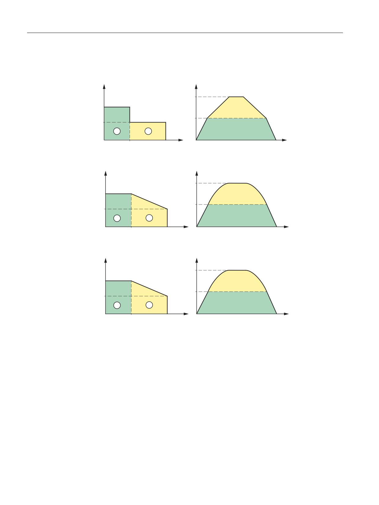
The following figures show the principal velocity and acceleration characteristic curves for the

respective types of characteristic curve:

• Constant torque characteristic (value = 0)

Y_PD[

D_PD[

Y_UHG

D_UHG

Y_UHG

Y_PD[

• Hyperbolic torque characteristic (value = 1)

Y_PD[

D_PD[

Y_UHG

D_UHG

Y_UHG

Y_PD[

• Linear torque characteristic (value = 2)

Y_PD[

D_PD[

Y_UHG

D_UHG

Y_UHG

Y_PD[

Characteristic parameters

The characteristic curve parameters result from the following machine data:

① Normal range

② Reducing range

v_max

$MA_MAX_AX_VELO

v_red

$MA_ACCEL_REDUCTION_SPEED_POINT * $MA_MAX_AX_VELO

a_max

$MA_MAX_AX_ACCEL

a_red

(1 - $MA_ACCEL_REDUCTION_FACTOR) * $MA_MAX_AX_ACCEL

Axes and spindles

120

Function Manual, 10/2020, 6FC5397-4GP40-0BA1

Acceleration and jerk

4.2 Detailed description

4.2.20.5

Programming: Channel-specific activation (DRIVE)

Functionality

The axis-specific velocity limit, above which the reduced acceleration acts as an axis for

traversing movements, is activated with the command DRIVE.

Syntax

DRIVE

Meaning

DRIVE:

Channel-specific switch-on of the reduced acceleration above the parameter-

ized velocity limit

G group:

Basic position:

MD20150 $MC_GCODE_RESET_VALUES[ 20 ]

Effectiveness:

Modal

Supplementary conditions

Characteristic changeover

If the acceleration reduction is active due to the programming of DRIVE and the acceleration

profile is changed over by SOFT or BRISK, traversing is then done with a substitute characteristic

with reduced dynamic limit values.

With the re-programming of DRIVE, the reduction in acceleration can be re-activated beyond

the parameterized velocity limit.

See also

Acceleration without jerk limitation (BRISK/BRISKA) (channel/axis-specific) (Page 81)

Jerk limitation with single-axis interpolation (SOFTA) (axis-specific) (Page 98)

4.3

Examples

4.3.1

Acceleration

4.3.1.1

Path velocity characteristic

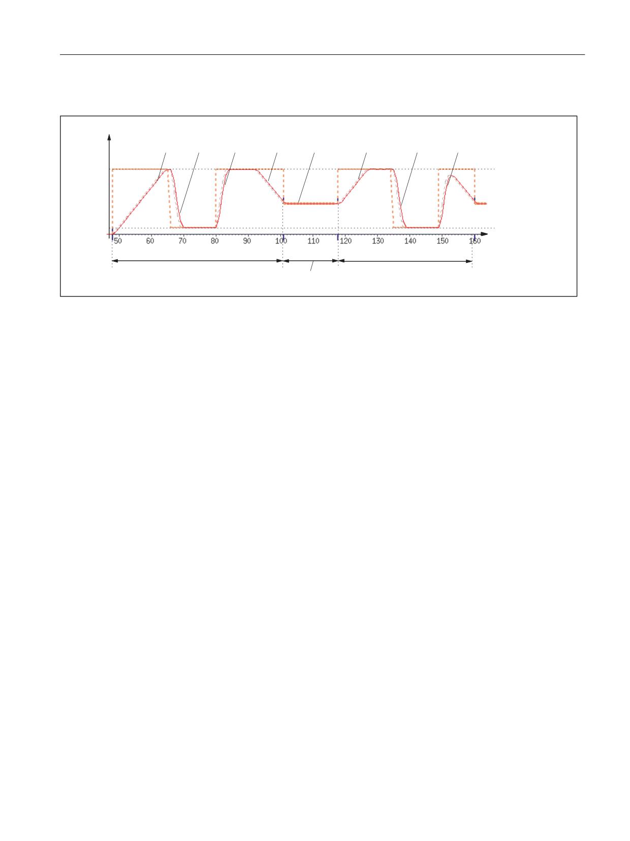
The following example shows the path velocity characteristic, based on programmed traversing

motion and the actions initiated in a part program segment.

Axes and spindles

Function Manual, 10/2020, 6FC5397-4GP40-0BA1

125

Acceleration and jerk

4.3 Examples

Part program extract

Program code

; Synchronized action: Acceleration switchover depending on fast input 1

($A_IN[1]):

N53 ID=1 WHEN $A_IN[1] == 1 DO $AC_PATHACC = 2.*$MA_MAX_AX_ACCEL[X]

; Synchronized action: Test override profile (simulation of external

interventions):

N54 ID=2 WHENEVER ($AC_TIMEC > 16) DO $AC_OVR=10

N55 ID=3 WHENEVER ($AC_TIMEC > 30) DO $AC_OVR=100

;Approach

N1000 G0 X0 Y0 BRISK

N1100 TRANS Y=-50

N1200 AROT Z=30 G642

; Contour

N2100 X0 Y0

N2200 X = 70 G1 F10000 RNDM=10 ACC[X]=30 ACC[Y]=30

N2300 Y = 70

N2400 X0

N2500 Y0

Axes and spindles

126

Function Manual, 10/2020, 6FC5397-4GP40-0BA1

Acceleration and jerk

4.3 Examples

Path velocity characteristic

Y >P V@

$&B295

W >

PV@

Acceleration profile: BRISK

Accelerate to 100% of path velocity (F10000) in accordance with acceleration default: ACC (N2200...)

Brake to 10% of path velocity as a result of override modification ($AC_OVR) in accordance with real-time acceleration

$AC_PATHACC (N53/N54...)

Accelerate to 100% of path velocity as a result of override modification ($AC_OVR) in accordance with real-time

acceleration $AC_PATHACC (N53/N55...)

Brake to block end velocity for intermediate smoothing block in accordance with acceleration default: ACC (N2200...)

Speed limitation as a result of smoothing (see 9)

Accelerate to 100% of path velocity ($AC_OVR) in accordance with acceleration default: ACC (N2300...)

Decelerate as a result of override modification at a rate of acceleration that is in accordance with real-time acceler-

ation $AC_PATHACC (N53/N54...)

Accelerate to 100% of path velocity as a result of override modification ($AC_OVR) in accordance with real-time

acceleration $AC_PATHACC (N53/N55...)

Intermediate block inserted within the control as a result of the programmed smoothing (RNDM) (N2200...)

Figure 4-9

Switching between path acceleration specified during preprocessing and real-time acceleration

4.3.2

Jerk

4.3.2.1

Path velocity characteristic

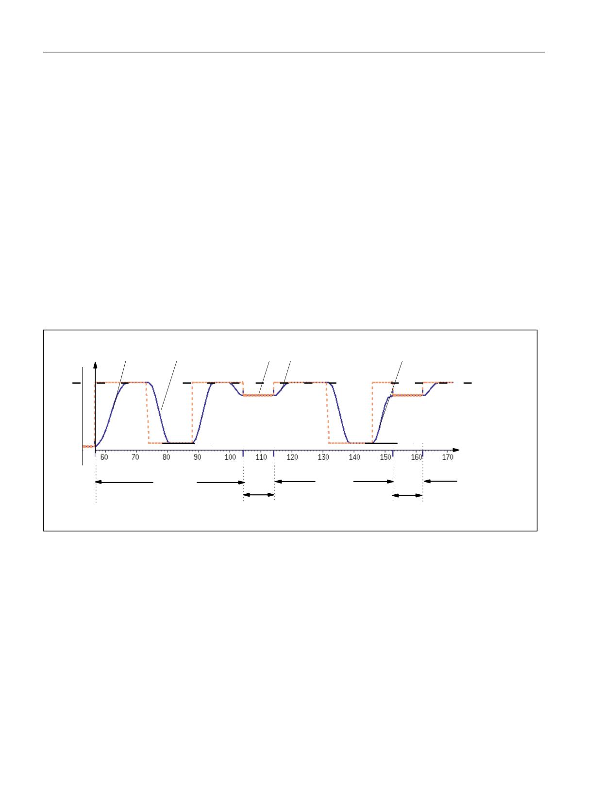
The following example shows the characteristic of path velocity and jerk based on programmed

traversing motion and the actions initiated in a part program segment.

Part program extract

Program code

; Setting of path acceleration and path jerk in the event of external

intervention:

N0100 $AC_PATHACC = 0.0

N0200 $AC_PATHJERK = 4.0 * ($MA_MAX_AX_JERK[X] + $MA_MAX_AX_JERK[Y]) / 2.0

Axes and spindles

Function Manual, 10/2020, 6FC5397-4GP40-0BA1

127

Acceleration and jerk

4.3 Examples

Program code

; Synchronized action: varying the override (simulation of external

interventions)

N0530 ID=1 WHENEVER ($AC_TIMEC > 16) DO $AC_OVR=10

N0540 ID=2 WHENEVER ($AC_TIMEC > 30) DO $AC_OVR=100

;Approach

N1000 G0 X0 Y0 SOFT

N1100 TRANS Y=-50

N1200 AROT Z=30 G642

; Contour

N2100 X0 Y0

N2200 X = 70 G1 F10000 RNDM=10

N2300 Y = 70

N2400 X0

N2500 Y0

Characteristic of path velocity and jerk

Y >P V@

295

W >

PV@

51'0

Acceleration profile: SOFT

Jerk according to $MA_MAX_AX_JERK[..]

Jerk according to $AC_PATHJERK

Jerk according to $MA_MAX_AX_JERK[..] (approach block end velocity)

Velocity limiting using arcs

Jerk according to $AC_PATHJERK

Figure 4-10

Switching between path jerk specified during preprocessing and $AC_PATHJERK

Axes and spindles

128

Function Manual, 10/2020, 6FC5397-4GP40-0BA1

Acceleration and jerk

4.3 Examples

4.3.3

Acceleration and jerk

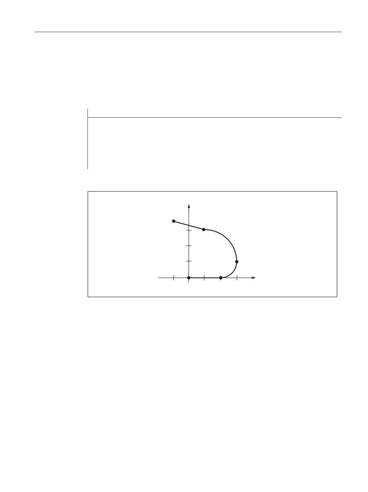
The following example shows the characteristic of velocity and acceleration of the X axis based

on the programmed traversing motion of the part program extract. Further, which of the

velocity and acceleration-relevant machine data are decisive for which section of the contour.

Part program extract

Program code

Comment

N90 F5000 SOFT G64

; Continuous-path mode, jerk-limited acceleration

N100 G0 X0 Y0 Z0

; Rapid traverse

N110 G1 X10

; Straight line

N120 G3 CR=5 X15 Y5

; Circular arc, radius 5 mm, block transition: Tangential

N130 G3 CR=10 X5 Y15

; Circular arc, radius 10 mm, block transition: Tangential

N140 G1 X-5 Y17.679

; Straight line, 15° kink

Contour

[

Figure 4-11

Contour of the part program extract

Axes and spindles

Function Manual, 10/2020, 6FC5397-4GP40-0BA1

129

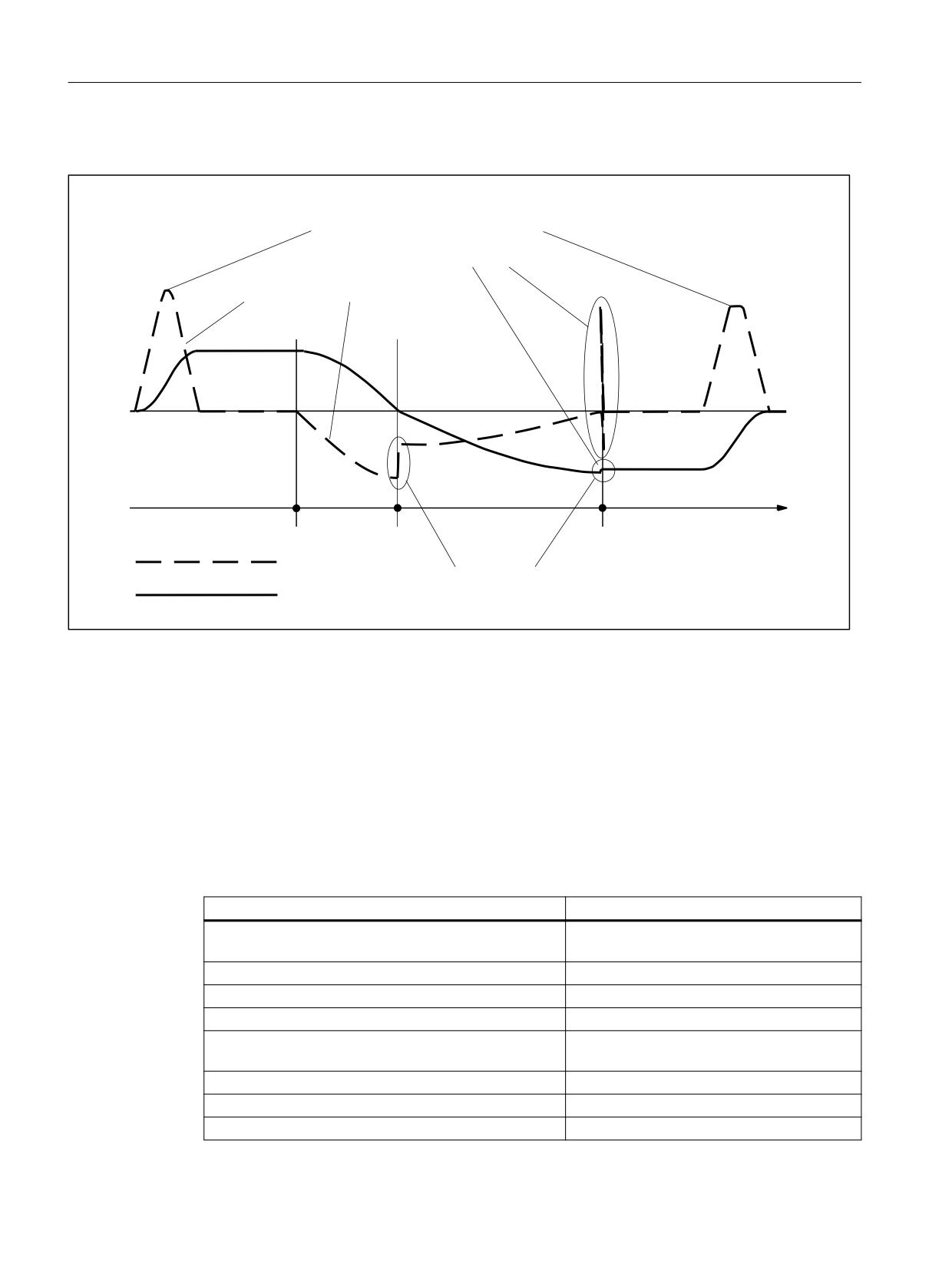
Acceleration and jerk

4.3 Examples

Velocity and acceleration characteristic

0$;B$;B$&&(/>;@

62)7B$&&(/B)$&725>;@

0$;B$&&(/B29/B)$&725>;@

0$;B$;B-(5.>;@

$[OH DFFHOHUDWLRQ

$[LV YHORFLW\

3$7+B75$16B-(5.B/,0>;@

Figure 4-12

Velocity and acceleration characteristic curves X axis

4.3.4

Knee-shaped acceleration characteristic

4.3.4.1

Activation

The example illustrates how the knee-shaped acceleration characteristic curve is activated on

the basis of the machine data and a part program extract.

Machine data

Value

MD35220 $MA_ACCEL_REDUCTION_SPEED_POINT[

= 0.4

MD35230 $MA_ACCEL_REDUCTION_FACTOR[X]

= 0.85

MD35242 $MA_ACCEL_REDUCTION_TYPE[X]

= 2

MD35240 $MA_ACCEL_TYPE_DRIVE[X]

= TRUE

MD35220

= 0.0

$MA_ACCEL_REDUCTION_SPEED_POINT[Y]

MD35230 $MA_ACCEL_REDUCTION_FACTOR[Y]

= 0.6

MD35242 $MA_ACCEL_REDUCTION_TYPE[Y]

= 1

MD35240 $MA_ACCEL_TYPE_DRIVE[Y]

= TRUE

Axes and spindles

130

Function Manual, 10/2020, 6FC5397-4GP40-0BA1

Acceleration and jerk

4.4 Data lists

Machine data

Value

MD35220

= 0.6

$MA_ACCEL_REDUCTION_SPEED_POINT[Z]

MD35230 $MA_ACCEL_REDUCTION_FACTOR[Z]

= 0.4

MD35242 $MA_ACCEL_REDUCTION_TYPE[Z]

= 0

MD35240 $MA_ACCEL_TYPE_DRIVE[Z]

= FALSE

Activation by entering as channel-specific initial setting:

MC_GCODE_RESET_VALUE[20] = 3 (DRIVE)

Part program extract

Program code

Comment

N10 G1 X100 Y50 Z50 F700

; Path motion (X,Y, Z) with DRIVE

N15 Z20

; Path motion (Z) with DRIVE

N20 BRISK

; Switchover to BRISK

N25 G1 X120 Y70

; Path motion (Y, Z) with substitute

characteristic curve

N30 Z100

; Path motion (Z) with BRISK

N35 POS[X] = 200 FA[X] = 500

; Positioning motion (X) with DRIVEA

N40 BRISKA(Z)

; Activate BRISKA for Z

N40 POS[Z] = 50 FA[Z] = 200

; Positioning motion (Z) with BRISKA

N45 DRIVEA(Z)

; Activate DRIVEA for Z

N50 POS[Z] = 100

; Positioning motion (Z) with DRIVE

N55 BRISKA(X)

; results in error message

4.4

Data lists

4.4.1

Machine data

4.4.1.1

NC-specific machine data

Number Identifier: $MN_

Description

18960

POS_DYN_MODE

Type of positioning axis dynamic response

4.4.1.2

Channel-specific machine data

Number

Identifier: $MC_

Description

20150

GCODE_RESET_VALUES

Initial setting of the G groups

20500

CONST_VELO_MIN_TIME

Minimum time with constant velocity

Axes and spindles

Function Manual, 10/2020, 6FC5397-4GP40-0BA1

131

Acceleration and jerk

4.4 Data lists

Number

Identifier: $MC_

Description

20600

MAX_PATH_JERK

Path-related maximum jerk

20602

CURV_EFFECT_ON_PATH_ACCEL

Influence of path curvature on path dynamic response

20610

ADD_MOVE_ACCEL_RESERVE

Acceleration reserve for overlaid motions

21158

JOG_JERK_ORI

Maximum jerk of the orientation axes when traversing in JOG

21159

JOG_JERK_ORI_ENABLE

Initial setting of the channel-specific jerk limitation of orien-

tation axes for traversing in JOG mode

21166

JOG_ACCEL_GEO

Maximum acceleration rate of the geometry axes when tra-

versing in JOG

21168

JOG_JERK_GEO

Maximum jerk of the geometry axes when traversing in JOG

4.4.1.3

Axis/spindlespecific machine data

Number

Identifier: $MA_

Description

32000

MAX_AX_VELO

Maximum axis velocity

32300

MAX_AX_ACCEL

Maximum axis acceleration

32310

MAX_ACCEL_OVL_FACTOR

Overload factor for velocity jump

32320

DYN_LIMIT_RESET_MASK

Reset behavior of dynamic limits

32400

AX_JERK_ENABLE

Axial jerk limitation

32402

AX_JERK_MODE

Filter type for axial jerk limitation

32407

AX_JERK_FIR_FREQ

Corner frequency axial jerk filter, type 5

32408

AX_JERK_FIR_ORDER

Filter order, axial jerk filter, type 5

32409

AX_JERK_FIR_WINDOW

Window type, axial jerk filter, type 5

32410

AX_JERK_TIME

Time constant for axial jerk filter

32411

AX_JERK_TIME_ADD

Time constant for the second axial jerk filter, type 4

32412

AX_JERK_FREQ

Blocking frequency of the axial jerk filter

32414

AX_JERK_DAMP

Damping, axial jerk filter

32420

JOG_AND_POS_JERK_ENABLE

Basic setting for axial jerk limitation

32430

JOG_AND_POS_MAX_JERK

Axial jerk for single axis motion

32431

MAX_AX_JERK

Maximum axial jerk at the block change in continuous-

path mode

32432

PATH_TRANS_JERK_LIM

Max. axial jerk of a geometry axis at block boundary

32433

SOFT_ACCEL_FACTOR

Scaling of acceleration limitation for SOFT

32434

G00_ACCEL_FACTOR

Scaling of acceleration limitation for G0

32435

G00_JERK_FACTOR

Scaling of axial jerk limitation for G0

32437

AX_JERK_VEL0

First velocity threshold for velocity-dependent jerk adap-

tation

32438

AX_JERK_VEL1

Second velocity threshold for the velocity-dependent

jerk adaptation

32439

MAX_AX_JERK_FACTOR

Factor to set the maximum jerk for higher velocities (ve-

locity-dependent jerk adaptation)

35220

ACCEL_REDUCTION_SPEED_POINT

Speed for reduced acceleration

35230

ACCEL_REDUCTION_FACTOR

Reduced acceleration

Axes and spindles

132

Function Manual, 10/2020, 6FC5397-4GP40-0BA1

Acceleration and jerk

4.4 Data lists

Number

Identifier: $MA_

Description

35240

ACCEL_TYPE_DRIVE

DRIVE acceleration characteristic for axes on/off

35242

ACCEL_REDUCTION_TYPE

Type of acceleration reduction

4.4.2

Setting data

4.4.2.1

Channelspecific setting data

Number

Identifier: $SC_

Description

42500

SD_MAX_PATH_ACCEL

Max. path acceleration

42502

IS_SD_MAX_PATH_ACCEL

Analysis of SD 42500: ON/OFF

42510

SD_MAX_PATH_JERK

Max. path-related jerk

42512

IS_SD_MAX_PATH_JERK

Analysis of SD 42510: ON/OFF

4.4.3

System variables

Identifier

Description

$AC_PATHACC

Path acceleration for real-time events

$AC_PATHJERK

Path jerk for real-time events

Axes and spindles

Function Manual, 10/2020, 6FC5397-4GP40-0BA1

133

Velocities, setpoint/actual value systems, closed-

loop control

5.1

Brief description

The description of functions explains how to parameterize a machine axis in relation to:

• Actual-value/measuring systems

• Setpoint system

• Operating accuracy

• Travel ranges

• Axis velocities

• Control parameters

5.2

Velocities, traversing ranges, accuracies

5.2.1

Velocities

Maximum path and axis velocities and spindle speed

The maximum path and axis velocities and spindle speed are influenced by the machine design,

the dynamic response of the drive and the limit frequency of the actual-value acquisition

(encoder limit frequency).

The maximum axis velocity is defined in machine data:

MD32000 $MA_MAX_AX_VELO (maximum axis velocity)

The maximum permissible spindle speed is specified using machine data:

MD35100 $MA_SPIND_VELO_LIMIT (maximum spindle speed)

For explanations, see Section "Spindles (Page 377)".

With a higher feedrate (resulting from programmed feedrates and feedrate override), the

velocity is limited to V_max.

This automatic feedrate limiting can lead to a drop in velocity over several blocks with programs

generated by CAD systems with extremely short blocks.

Axes and spindles

Function Manual, 10/2020, 6FC5397-4GP40-0BA1

135

Velocities, setpoint/actual value systems, closed-loop control

5.2 Velocities, traversing ranges, accuracies

Example:

Interpolation cycle = 12 ms

N10 G0 X0 Y0; [mm]

N20 G0 X100 Y100; [mm]

⇒ Path length programmed in block = 141.42 mm

⇒ V_max= (141.42 mm/12 ms) _* 0.9 = 10606.6 mm/s = 636.39 m/min

Minimum path, axis velocity

The following restriction applies to the minimum path or axis velocity:

9PLQ

ุ

,QFU

&RPSXWDWLRQDO >

PP RU GHJUHHV

,32 F\FOH >V@

UHVROXWLRQ

The computational resolution is defined using machine data:

MD10200 $MN_INT_INCR_PER_MM (computational resolution for linear positions)

MD10210 $MN_INT_INCR_PER_DEG (computational resolution for angular positions)

If V_minis not reached, no traversing is carried out.

Example:

MD10200 $MN_INT_INCR_PER_MM = 1000 [incr/mm] ;

Interpolation cycle = 12 ms;

⇒ V_min = 10^-3/(1000 ^incr/_mm x 12 ms) = 0.005 ^mm/_min;

The value range of the feedrates depends on the computational resolution selected.

For the standard assignment of machine data:

MD10200 $MN_INT_INCR_PER_MM

(computational resolution for linear positions) (1000 incr./mm)

MD10210 $MN_INT_INCR_PER_DEG

(computational resolution for angular positions) (1000 incr./deg.)

The following value range can be programmed with the specified resolution:

Range of values for path feed F and geometry axes:

Metric system:

Inch system:

0.001 ≤ F ≤ 999,999.999

0.001 ≤ F ≤ 399,999.999 [inch/min, inch/rev]

[mm/min, mm/rev, degrees/min, degrees/rev]

Axes and spindles

136

Function Manual, 10/2020, 6FC5397-4GP40-0BA1

Velocities, setpoint/actual value systems, closed-loop control

5.2 Velocities, traversing ranges, accuracies

Range of values for feedrate for positioning axes:

Metric system:

Inch system:

0.001 ≤ FA ≤ 999,999.999

0.001 ≤ FA ≤ 399,999.999

[mm/min, mm/rev, degrees/min, degrees/rev]

[inch/min, inch/rev]

Range of values for spindle speed S:

0.001 ≤ S ≤ 999,999.999 [rpm]

If the computational resolution is increased/decreased by a factor, then the value ranges change

accordingly.

5.2.2

Traversing ranges

Range of values of the traversing ranges

The range of values of the traversing range depends on the computational resolution selected.

For the standard assignment of machine data:

MD10200 $MN_INT_INCR_PER_MM

(computational resolution for linear positions) (1000 incr./mm)

MD10210 $MN_INT_INCR_PER_DEG

(computational resolution for angular positions) (1000 incr./deg.)

The following value range can be programmed with the specified resolution:

Table 5-1

Traversing ranges of axes

G71 [mm, degrees]

G70 [inch, degrees]

Range

Linear axes X, Y, Z, etc.

∓ 999,999.999

∓ 399,999.999

Rotary axes A, B, C, etc.

∓ 999,999.999

Interpolation parameters I, J, K

∓ 999,999.999

∓ 399,999.999

The unit of measurement of rotary axes is always degrees.

If the computational resolution is increased/decreased by a factor of 10, the ranges of values

change accordingly.

The traversing range can be limited by software limit switches and work areas (see Function

Manual Monitoring and Compensations, Section Axis monitoring).

For special features for a large traversing range for linear and rotary axes, see Section "Homing

(Page 31)".

The traversing range for rotary axes can be limited via machine data.

Further information:

Axes and spindles

Function Manual, 10/2020, 6FC5397-4GP40-0BA1

137

Velocities, setpoint/actual value systems, closed-loop control

5.2 Velocities, traversing ranges, accuracies

Rotary axes (Page 307)

5.2.3

Positioning accuracy of the control system

Actual-value resolution and computational resolution

The positioning accuracy of the control depends on the actual-value resolution (=encoder

increments/(mm or degrees)) and the computational resolution (=internal increments/(mm or

degrees)).

The coarse resolution of these two values determines the positioning accuracy of the control.

The input resolution, interpolator and position-control cycle selections have no effect on this

accuracy.

As well as limiting using MD32000, the control limits the maximum path velocity in relation to

the situation and according to the following formula:

,QWHUQDO LQFUHPHQWV PP

(QFRGHU LQFUHPHQWV PP

(1&B5(62/ >Q@

(1&B38/6(B08/7>Q@

'5,9(B(1&B5$7,2B180(5$ >Q@

'5,9(B(1&B5$7,2B'(120 >Q@

'5,9(B$;B5$7,2B'(120 >Q@

'5,9(B$;B5$7,2B180(5$ >Q@

/($'6&5(:B3,7&+

,17B,1&5B3(5B00

5.2.4

Input/display resolution, computational resolution

Resolutions: Differences

Resolutions, e.g. resolutions of linear and angular positions, velocities, accelerations and jerk,

must be differentiated as follows:

• Input resolution

Data is input via the control panel or part programs.

• Display resolution

Data is displayed via the operator panel front.

• Computational resolution

Data input via the control panel or part program is displayed internally.

Axes and spindles

138

Function Manual, 10/2020, 6FC5397-4GP40-0BA1

Velocities, setpoint/actual value systems, closed-loop control

5.2 Velocities, traversing ranges, accuracies

The input and display resolution is determined by the specified operator panel front used,

whereby the display resolution for position values with the machine data:

MD9004 $MM_DISPLAY_RESOLUTION (display resolution)

can be changed.

The machine data:

MD9011 $MM_DISPLAY_RESOLUTION_INCH (display resolution in inch)

can be used to configure the display resolution for position values with inch setting.

This allows you to display up to six decimal places with the inch setting.

For the programming in part programs, the input resolutions listed in the NC Programming

Programming Manual apply.

The desired computational resolution is defined using the machine data:

MD10200 $MN_INT_INCR_PER_MM (calculation resolution for linear positions)

and

MD10210 $MN_INT_INCR_PER_ DEG (calculation resolution for angular positions)

It is independent of the input/display resolution but should have at least the same resolution.

The maximum number of places after the decimal point for position values, velocities, etc., in

the part program and the number of places after the decimal point for tool offsets, work offsets,

etc. (and therefore also for the maximum possible accuracy) is defined by the computational

resolution.

The accuracy of angle and linear positions is limited to the computational resolution by rounding

the product of the programmed value with the computational resolution to an integer number.

To make the rounding clear, powers of 10 should be used for the calculation resolution.

Example of rounding:

Computational resolution: 1000 increments / mm

Programmed path: 97.3786 mm

Effective value = 97.379 mm

Example of programming in the ¹/₁₀ μm range:

All the linear axes of a machine are to be programmed and traversed within the range of values

0.1 to 1000 μm.

⇒ In order to position accurately to 0.1 μm, the computational resolution must be set to ≥ 10⁴

incr./mm.

⇒ MD10200 $MN_INT_INCR_PER_MM = 10000 [incr./mm]:

Axes and spindles

Function Manual, 10/2020, 6FC5397-4GP40-0BA1

139

Velocities, setpoint/actual value systems, closed-loop control

5.2 Velocities, traversing ranges, accuracies

⇒ Example of associated part program:

Program code

Comment

N20 G0 X1.0000 Y1.0000

; Axes move to position X=1.0000 mm, Y=1.0000 mm

N25 G0 X5.0002 Y2.0003

; Axes move to position X=5.0002 mm, Y=2.0003 mm

5.2.5

Scaling of physical quantities of machine and setting data

Input/output units

Machine and setting data with a physical unit are interpreted in the input/output units stated

below depending on whether the metric or inch system is selected:

Physical unit

Input/output units for standard basic system

Metric

Inch

Linear position

1 mm

1 inch

Angular position

1 degree

Linear velocity

1 mm/min

1 inch/min

Angular velocity

1 rpm

Linear acceleration

1 m/s²

1 inch/s²

Angular acceleration

1 rev./^s2

1 rev./s²

Linear jerk

1 m/s³

1 inch/s³

Angular jerk

1 rev./s³

Time

1 s

Position controller servo gain

1/s

Revolutional feedrate

1 mm/rev

inch/rev

Compensation value linear position

1 mm

1 inch

Compensation value angular position

1 degree

Internally in the control, the following units are used, whatever basic system is selected:

Physical unit

Unit

Linear position

1 mm

Angular position

1 degree

Linear velocity

1 mm/s

Angular velocity

1 deg./s

Linear acceleration

1 mm/s²

Angular acceleration

1 degree/s²

Linear jerk

1 mm/s³

Angular jerk

1 degree/s³

Time

1 s

Position controller servo gain

1/s

Revolutional feedrate

1 mm/degree

Axes and spindles

140

Function Manual, 10/2020, 6FC5397-4GP40-0BA1

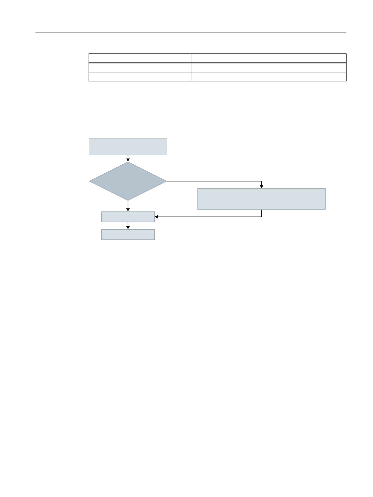
Velocities, setpoint/actual value systems, closed-loop control

5.2 Velocities, traversing ranges, accuracies

Physical unit

Unit

Compensation value linear position

1 mm

Compensation value angular position

1 degree

The user can define different input/output units for machine and setting data. This also requires

an adjustment between the newly selected input/output units and the internal units via the

following machine data:

• MD10220 $MN_SCALING_USER_DEF_MASK

• MD10230 $MN_SCALING_FACTORS_USER_DEF[n]

,QSXW RXWSXW XQLWV IRU PDFKLQH DQG

VHWWLQJ GDWD

'R WKH LQSXW RXWSXW

XQLWV FRUUHVSRQG WR WKH VWDQGDUG

EDVLF V\VWHP"

8VHU GHILQHG

6&$/,1*B)$&7256B86(5B'()>Q@

<HV

6&$/,1*B)$&7256B86(5B'()B0$6.

)RUPDW FRQYHUVLRQ

,QWHUQDO XQLWV

The following applies:

Selected I/O unit = (MD10230 $MN_SCALING_FACTORS_USER_DEF[n]) * internal unit

The selected I/O unit, expressed in the internal units 1 mm, 1 degree, and 1 s must therefore be

entered in machine data MD10230 $MN_SCALING_FACTORS_USER_DEF[n].

Example 1:

Machine data input/output of the linear velocities is to be in m/min instead of mm/min (initial

state).

(The internal unit is mm/s)

⇒ The scaling factor for the linear velocities is to differ from the standard setting. For this,

in machine data:

MD10220 $MN_SCALING_USER_DEF_MASK

bit number 2 must be set.

⇒ MD10220 $MN_SCALING_USER_DEF_MASK = 'H4'; (bit no. 2 as hex value)

⇒ The scaling factor for the linear velocities is to differ from the standard setting. For this,

in machine data:

MD10220 $MN_SCALING_USER_DEF_MASK

bit number 2 must be set.

⇒ MD10220 $MN_SCALING_USER_DEF_MASK = 'H4'; (bit no. 2 as hex value)

Axes and spindles

Function Manual, 10/2020, 6FC5397-4GP40-0BA1

141

Velocities, setpoint/actual value systems, closed-loop control

5.3 System of units, metric/inch

⇒ The scaling factor is calculated using the following formula:

6HOHFWHG LQSXW RXWSXW XQLW

6&$/,1*B)$&7256B86(5B'()>Q@

,QWHUQDO XQLW

PLQ

6&$/,1*B)$&7256B86(5B'()>Q@

ය

6&$/,1*B)$&7256B86(5B'()>Q@

Index n defines the "linear velocity" in the "Scaling factors of physical quantities" list.

Example 2:

In addition to the change in Example 1, the machine data input/output of linear accelerations

must be in ft/s² instead of m/s² (initial state).

(The internal unit is mm/s².)

ය 0'

6&$/,1*B86(5B'()B0$6.

%LW 1R DQG %LW 1R RI H[DPSOH DV D +H[ YDOXH

ය

6&$/,1*B)$&7256B86(5B'()> @

ය

6&$/,1*B)$&7256B86(5B'()> @

Index 4 defines the "linear acceleration" in the "Scaling factors of physical quantities" list.

5.3

System of units, metric/inch

5.3.1

Function

5.3.1.1

Parameterized and programmed system of units

SINUMERIK control systems can operate with a metric system of units as well as an inch system

of units.

Axes and spindles

142

Function Manual, 10/2020, 6FC5397-4GP40-0BA1

Velocities, setpoint/actual value systems, closed-loop control

5.3 System of units, metric/inch

Parameterized system of units (basic system)

The basic setting of the system of units (basic system) is set in machine data MD10240

$MN_SCALING_SYSTEM_IS_METRIC (see "Commissioning (Page 147)").

Depending on the basic system, all length-related data is interpreted either as metric or inch

system of units.

Metric system of units:

mm, mm/min, m/s2, m/s3, mm/rev.

Inch system of units:

inch, inch/min, inch/s2, inch/s3, inch/rev.

The basic system also defines the interpretation of the programmed F value for linear axes:

Feed type

Metric system of units

Inch system of units

G94

mm/min

inch/min

G95

mm/rev.

inch/rev.

Programmed system of units

Using the commands of G group 13 (system of units, inch/metric) within the part program, you

can toggle between the metric and inch system of units (see "Programming (Page 151)").

The programmed system of units and the basic system may be identical or different at any time.

Switchover of the system of units within a particular section of the part program could, for

example, be used to machine an inch thread on a workpiece within a metric basic system.

The reset setting of the G group is defined in machine data MD20150

$MC_GCODE_RESET_VALUES (see "Commissioning (Page 147)").

HMI display

Data relating to length is displayed as follows on the user interface:

Display

in the basic system

in the programmed system of

units

Machine data

Data in the machine coordinate

system

Tool data

Work offsets

Data in the workpiece coordinate

system

NC/PLC interface

In the case of NC/PLC interface signals containing dimension information, e.g. feedrate for path

and positioning axes, data exchange is carried out with the PLC in the configured basic system.

Axes and spindles

Function Manual, 10/2020, 6FC5397-4GP40-0BA1

143

Velocities, setpoint/actual value systems, closed-loop control

5.3 System of units, metric/inch

Reading in external part programs

If part programs, including data sets (work offsets, tool offsets, etc.), programmed in a system

of units other than the basic system are read in from an external source, then the basic system

must first be changed.

5.3.1.2

Extended system of units functionality

From SW 5 and higher, the system of units functionality has been extended, which significantly

simplifies toggling between systems of units.

The functions include:

• New G commands G700/G710 (see "Programming (Page 151)")

• Data backup with system of units identifier INCH/METRIC (see "Commissioning (Page 147)")

• Automatic data conversions when the system of units is changed, e.g. for:

- Work offsets

- Compensation data (EEC, QEC)

- Tool offsets

- ...

For compatibility reasons, the extended system of units functionality must be activated using a

machine data (see "Commissioning (Page 147)").

5.3.1.3

Extended system of units functionality

From SW 5 and higher, the system of units functionality has been extended, which significantly

simplifies toggling between systems of units.

The functions include:

• System of units switchover at the user interface (Page 145)

• New G commands G700/G710 (see "Programming (Page 151)")

• Data backup with system of units identifier INCH/METRIC (see "Commissioning (Page 147)")

• Automatic data conversions when the system of units is changed, e.g. for:

- Work offsets

- Compensation data (EEC, QEC)

- Tool offsets

- ...

For compatibility reasons, the extended system of units functionality must be activated using a

machine data (see "Commissioning (Page 147)").

Axes and spindles

144

Function Manual, 10/2020, 6FC5397-4GP40-0BA1

Velocities, setpoint/actual value systems, closed-loop control

5.3 System of units, metric/inch

5.3.1.4

System of units switchover at the user interface

Requirement

Extended system of units functionality is active (MD10260 $MN_CONVERT_SCALING_SYSTEM

= 1; see "Commissioning (Page 147)")

Function

The relevant softkey on the HMI in the "Machine" operating area is used to change the system

of units of the control system.

The system of units is only switched over under the following conditions:

• MD20110 $MC_RESET_MODE_MASK, bit 0 is set in every channel.

• All channels are in the Reset state.

• Axes do not currently traverse with JOG, DRF, or PLC.

• Constant grinding wheel peripheral speed (GWPS) is not active.

Actions such as part program start or mode change are disabled while the system of units is

being switched over.

The actual change in the system of units is made by writing all the necessary machine data and

subsequently activating them.

The following machine data are automatically switched over consistently for all configured

channels:

• MD10240 $MN_SCALING_SYSTEM_IS_METRIC

• MD20150 $MN_GCODE_RESET_VALUES

Reset position

When the system of units is switched over from the user interface, the reset position of the G

group 13 is automatically adapted to the actual system of units:

MD20150 $MC_GCODE_RESET_VALUES[12] = <actual system of units>

NCU link

Note

If several NCUs are linked by NCU link, the switchover has the same effect on all linked NCUs. If

the requirements for a switchover are not fulfilled on one of the connected NCUs, no switchover

will take place on any of the NCUs. It is assumed that when there is a NCU link, interpolations

between several NCUs will take place on the existing NCUs, whereby the interpolations can

provide correct results only if the same systems of units are used.

Further information:

Function Manual Basic Functions; Distributed systems

Axes and spindles

Function Manual, 10/2020, 6FC5397-4GP40-0BA1

145

Velocities, setpoint/actual value systems, closed-loop control

5.3 System of units, metric/inch

System data

When the system of units is switched over, from the user's viewpoint, all length-related

specifications are converted to the new system of units automatically.

This includes:

• Positions

• Feedrates

• Accelerations

• Jerk

• Tool offsets

• Programmable, adjustable and external work offsets and DRF offsets

• Compensation values

• Protection zones

• Machine data

• JOG and handwheel factors

After the switchover, all of the above mentioned data is available in physical quantities.

Data, for which no unique physical units are defined, is not converted automatically.

This includes:

• R parameters

• GUDs (Global User Data)

• LUDs (Local User Data)

• PUDs (Program global User Data)

• Analog inputs/outputs

• Data exchange via FC21

The user is prompted to take the currently valid system of units MD10240

$MN_SCALING_SYSTEM_IS_METRIC into consideration.

NC/PLC interface

The current system of units setting can be read at the NC/PLC interface using the following signal:

DB10 DBX107.7 (inch system of units)

The number of times that the system of units has been switched over since the last time the

control powered up can be read out using the following signal byte:

DB10 DBB71 (change counter, system of units inch/metric)

Starting value after the control powered up: 1

Axes and spindles

146

Function Manual, 10/2020, 6FC5397-4GP40-0BA1

Velocities, setpoint/actual value systems, closed-loop control

5.3 System of units, metric/inch

5.3.2

Commissioning

NC-specific machine data

Basic system

The basic system to be used by the controller for the scaling of length-dependent physical

variables for data input/output is specified via the machine data:

MD10240 $MN_SCALING_SYSTEM_IS_METRIC

Value

Meaning

0 (= FALSE)

Data relating to length is interpreted as inch data.

1 (= TRUE)

Data relating to length is interpreted as metric data.

The system must be powered up again after changing this machine data as otherwise associated

machine data, which have physical units, will be incorrectly scaled.

The following procedure must be complied with:

• Changing the MD using manual entry:

1. Power up the system.

–

2. Machine data with physical units: Enter a value.

• The MD is changed using machine data:

1. Power up the system.

–

2. Load the machine data file once again so that the new physical units are taken into

account.

When changing MD10240, Alarm 4070 "Normalizing machine data has been changed" is

output.

Note

When changing over the system of units at a control system, all length-related data must be

converted consistently and completely into the other measuring system.

Conversion factor (NC-specific)

The factor for converting from metric into the inch system of units is set in machine data:

MD10250 $MN_SCALING_VALUE_INCH (conversion factor for inch)

Default value: 25.4

The conversion factor becomes active when selecting the non-metric basic system (MD10240

$MN_SCALING_SYSTEM_IS_METRIC = 0).

Axes and spindles

Function Manual, 10/2020, 6FC5397-4GP40-0BA1

147

Velocities, setpoint/actual value systems, closed-loop control

5.3 System of units, metric/inch

The following data are multiplied by the conversion factor:

• Length-related data for input/output (e.g. when uploading machine data, work offsets)

• Programmed F values for linear axes

• Programmed geometry of an axis (position, polynomial coefficients, radius for circle

programming, ...), if the system of units programmed with G70/G71 differs from the basic

system (MD10240 $MN_SCALING_SYSTEM_IS_METRIC).

Note

By changing the conversion factor, the control system can be adapted to customer-specific

systems of units.

Extended system of units functionality

The extended system of units functionality can be activated using the following compatibility

machine data:

MD10260 $MN_CONVERT_SCALING_SYSTEM

Value

Meaning

0 (= FALSE)

Extended system of units functionality not active (default setting; compati-

bility to previous software releases)

1 (= TRUE)

Extended system of units functionality active

When changing MD10240, Alarm 4070 "Normalizing machine data has been changed" is

output.

Data backup

Individual data sets that are read from the control system and contain data affected by the

system of units, are assigned an identifier during reading that indicates the current setting for

the system of units:

• MD10260 $MN_CONVERT_SCALING_SYSTEM

• MD10240 $MN_SCALING_SYSTEM_IS_METRIC

The identifier records in which system of units the data have been read out. This ensures that no

data sets are read into the control with a system of units other than that which is currently set.

Since the identifier is also evaluated in part programs, these can also be "protected" against

operator errors as described above. You can therefore prevent part programs containing, e.g.

only metric data, from running on an inch system of units.

Archive and machine data sets are downward-compatible with the following setting:

MD11220 $MN_INI_FILE_MODE = 2

Note

The INCH/METRIC identifier is only generated if the compatibility machine data:

MD10260 $MN_CONVERT_SCALING_SYSTEM = TRUE

Axes and spindles

148

Function Manual, 10/2020, 6FC5397-4GP40-0BA1

Velocities, setpoint/actual value systems, closed-loop control

5.3 System of units, metric/inch

Note

Rounding machine data

All length-related machine data is rounded to the nearest 1 pm when writing in the inch system

of units (MD10240 $MN_SCALING_SYSTEM_IS_METRIC=0 and MD10260

$MN_CONVERT_SCALING_SYSTEM=1), to avoid rounding problems.

This corrects the loss of accuracy resulting from conversion to ASCII when reading out a data

backup in the inch system of units when the data is read back into the system.

Input resolution and computational resolution

The input and calculation resolution is defined as an internal number of increments per

millimeter.

MD10200 $MN_INT_INCR_PER_MM

The precision of entry of linear positions is limited to the calculation resolution. The product of

the programmed position value and the calculation resolution is rounded up to the next integer.

To make the rounding clear and understandable, powers of 10 should be used for the calculation

resolution.

Example:

1 inch = 25.4 mm ⇒ 0.0001 inch = 0.00254 mm = 2.54 μm = 2540 nm

To be able to program and display the last 40 nm, a value of 100000 must be parameterized for

the input and calculation resolution.

Only with this identical setting for both systems of units is it possible to change the system of

units without a significant loss of accuracy. Once MD10200 has been set to this value, it will not

need to be changed each time the measuring system is switched over.

System of units for positioning tables

The system of units for positional data of the indexing axis tables and switching points for

software cams is configured in machine data:

MD10270 $MN_POS_TAB_SCALING_SYSTEM

Further information:

Function Manual Axis and Spindles; Software cams, position switching signals and indexing axes

User tool data

The physical units for user-defined tool and tool cutting edge data can be set in the following

machine data:

• MD10290 $MN_CC_TDA_PARAM_UNIT

• MD10292 $MN_CC_TOA_PARAM_UNIT

Note

When the system of units is switched over, all length-related tool data is converted to the new

system of units.

Axes and spindles

Function Manual, 10/2020, 6FC5397-4GP40-0BA1

149

Velocities, setpoint/actual value systems, closed-loop control

5.3 System of units, metric/inch

Channel-specific machine data

Reset position

For each channel, the reset position of G group 13 (system of units, inch/metric) is set in the

machine data:

MD20150 $MC_GCODE_RESET_VALUES[12] (reset position of G group 13)

Axis/spindle-specific machine data

Conversion factor (axis-specific)

To make pure positioning axes independent of G70/G71, a factor for converting from metric into

the inch system of units can be set in machine data:

MD31200 $MA_SCALING_FACTOR_G70_G71 (conversion factor when G70/G71 is active)

Default value: 25.4

Note

The conversion factor should be identical for all three geometry axes.

JOG and handwheel factor

The following machine data comprises two values containing axis-specific increment weighting

factors for each of the two system of units:

MD31090 $MA_JOG_INCR_WEIGHT

Depending on the actual setting in MD10240 SCALING_SYSTEM_IS_METRIC, the control system

automatically selects the appropriate value.

The user defines the two increment factors when the system is commissioned.

Example: Increment evaluations for the 1st axis

• Metric:

MD31090 $MA_JOG_INCR_WEIGHT[ 0 ; AX1 ] = 0.001 mm

• Inch:

MD31090 $MA_JOG_INCR_WEIGHT[ 1 ; AX1 ] = 0.00254 mm ≙ 0.0001 inch

In this way, MD31090 does not have to be written at every inch/metric switchover.

Remaining distances are not accumulated during incremental traversing with JOG when the

system of units is changed, since all internal positions always refer to mm.

System of units for sag compensation

The system of units for sag compensation is configured using machine data:

MD32711 $MA_CEC_SCALING_SYSTEM_METRIC

Further information:

Function Manual Monitoring and Compensating; Compensations

Axes and spindles

150

Function Manual, 10/2020, 6FC5397-4GP40-0BA1

Velocities, setpoint/actual value systems, closed-loop control

5.3 System of units, metric/inch

5.3.3

Programming

5.3.3.1

Switching over the system of units (G70/G71/G700/G710)

Using the commands of G group 13 (inch/metric system of units) within a part program, you can

switch over between the metric and inch system of units.

Activation

In order that commands G700 and G710 are available, the extended system of units

functionality must be switched on (MD10260 $MN_CONVERT_SCALING_SYSTEM = 1).

Syntax

G70

G71

G700

G710

Meaning

G70:

Activating the inch system of units

The inch system of units is used to read and write geometrical data in units of length.

Technological data in units of length (e.g. feedrates, tool offsets, adjustable work offsets,

machine data and system variables) is read and written using the parameterized basic sys-

tem.

G group:

Initial setting:

Settable via MD20150 $MC_GCODE_RESET_VALUES

Effectiveness:

Modal

G71:

Activating the metric system of units

The metric system of units is used to read and write geometrical data in units of length.

Technological data in units of length (e.g. feedrates, tool offsets, adjustable work offsets,

machine data and system variables) is read and written using the parameterized basic sys-

tem.

G group:

Initial setting:

Settable via MD20150 $MC_GCODE_RESET_VALUES

Effectiveness:

Modal

G700:

Activating the inch system of units

All geometrical and technological data in units of length is read and written using the inch

system of units.

G group:

Initial setting:

Settable via MD20150 $MC_GCODE_RESET_VALUES

Effectiveness:

Modal

Axes and spindles

Function Manual, 10/2020, 6FC5397-4GP40-0BA1

151

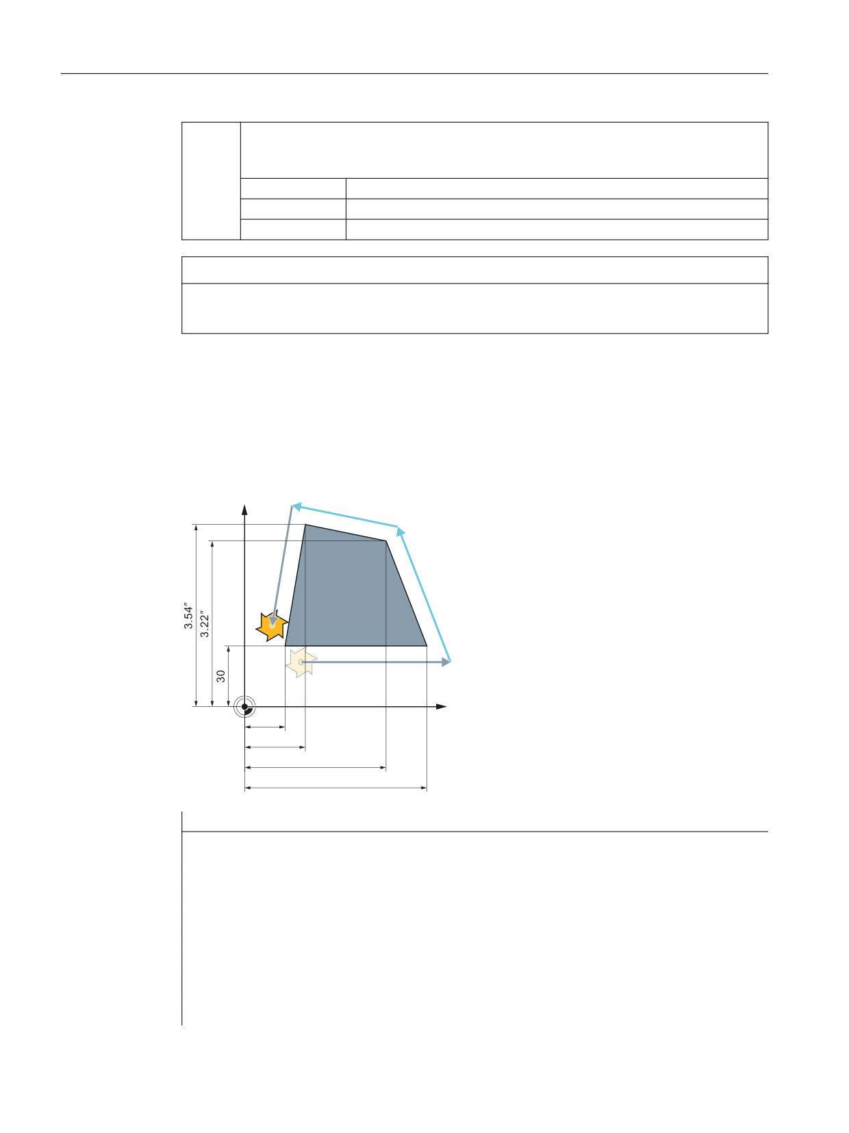
Velocities, setpoint/actual value systems, closed-loop control

5.3 System of units, metric/inch

G710:

Activating the metric system of units

All geometrical and technological data in units of length is read and written using the metric

system of units.

G group:

Initial setting:

Settable via MD20150 $MC_GCODE_RESET_VALUES

Effectiveness:

Modal

NOTICE

Axis-specific data of rotary axes

Axis-specific data of rotary axes is read and written using the parameterized basic system.

Example

The basic system is metric (MD10240 $MN_SCALING_SYSTEM_IS_METRIC = 1). However, the

workpiece drawing has dimensions shown in inches. This is the reason why within the part

program, the inch system of units is selected. After the inch dimensions have been processed,

the metric system of units is again selected.

;

ೀ

Program code

Comment

N10 G0 G90 X20 Y30 Z2 S2000 M3 T1

; X=20 mm, Y=30 mm, Z=2 mm, F=rapid traverse

mm/min

N20 G1 Z-5 F500

; Z=-5 mm, F=500 mm/min

N30 X90

; X=90 mm

N40 G70 X2.75 Y3.22

; programmed system of units: inch

; X=2.75 inch, Y=3.22 inch, F=500 mm/min

N50 X1.18 Y3.54

; X=1.18 inch, Y=3.54 inch, F=500 mm/min

N60 G71 X20 Y30

; programmed system of units: Metric

; X=20 mm, Y=30 mm, F=500 mm/min

N70 G0 Z2

; Z=2 mm, F=rapid traverse mm/min

Axes and spindles

152

Function Manual, 10/2020, 6FC5397-4GP40-0BA1

Velocities, setpoint/actual value systems, closed-loop control

5.3 System of units, metric/inch

Program code

Comment

N80 M30

; end of program

Further information

Reading and writing data in the case of G70/G71 and G700/G710

Data area

G70 / G71

G700 / G710

Read

Write

Read

Write

Display, decimal places (WCS)

Display, decimal places (MCS)

Feedrates

Position data X, Y, Z

Interpolation parameters I, J, K

Circle radius (CR)

Polar radius (RP)

Thread pitch

Programmable FRAME

Settable FRAMES

Basic frames

External work offsets

Axial preset offset

Working area limits (G25/G26)

Protection areas

Tool offsets

Length-related machine data

Length-related setting data

Length-related system variables

GUDs

LUDs

PUDs

R parameters

Siemens cycles

Jog/handwheel increment factor

P: Writing/reading is performed in the programmed system of units.

G: Writing/reading is performed in the configured basic system

Synchronized actions

Note

Reading position data in synchronized actions

If a system of units has not been explicitly programmed in the synchronized action (condition

component and/or action component) length-related position data in the synchronized action

will always be read in the parameterized basic system.

Axes and spindles

Function Manual, 10/2020, 6FC5397-4GP40-0BA1

153

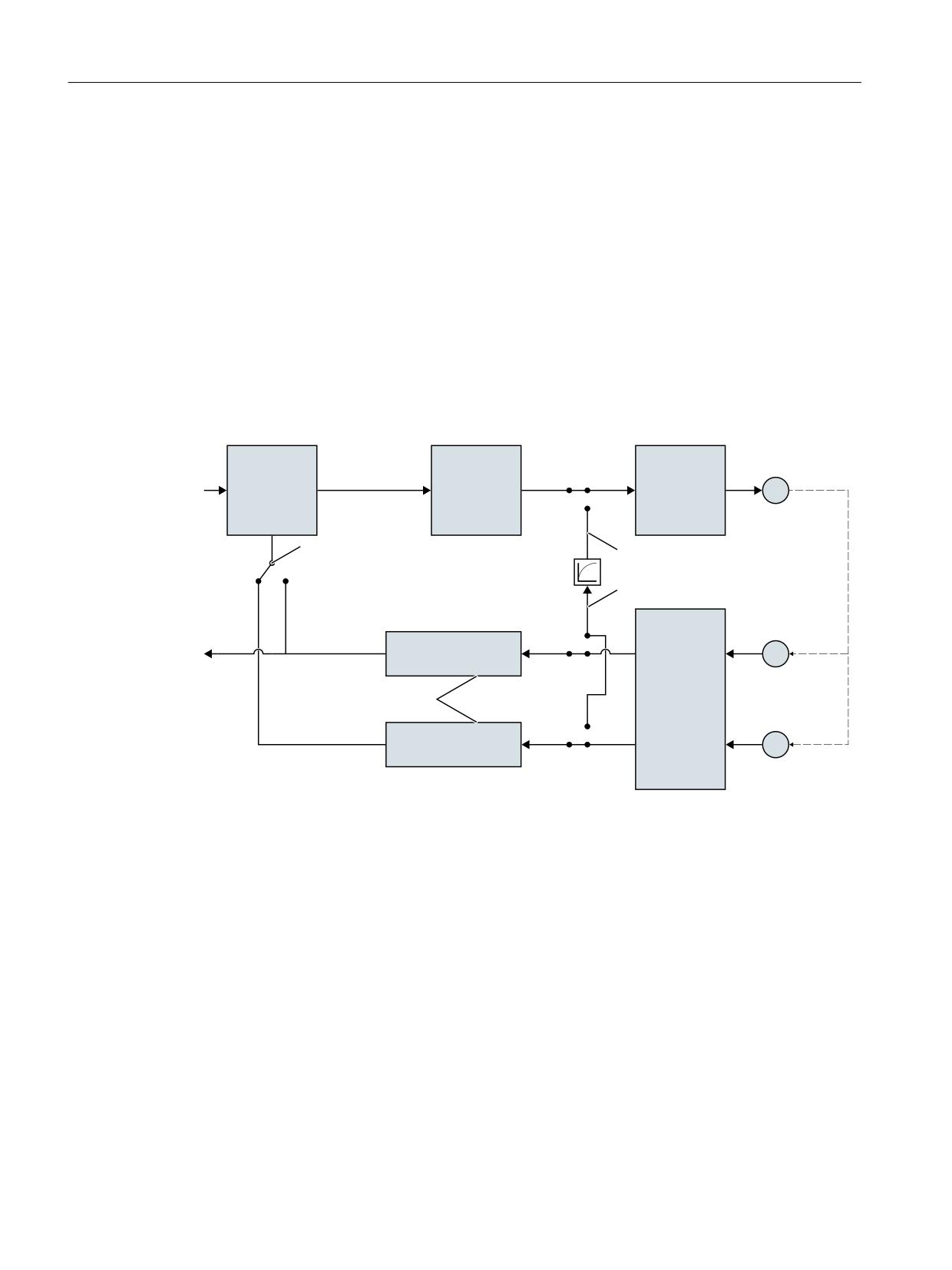
Velocities, setpoint/actual value systems, closed-loop control

5.4 Setpoint/actual-value system

Further information: Function Manual, Synchronized Actions

5.4

Setpoint/actual-value system

5.4.1

General information

Control loop

A control loop with the following structure can be configured for every closed-loop controlled

axis/spindle:

6SHHG

&ORVHG ORRS

VHWSRLQW

FRQWURO

RXWSXW

PDUVKDOOLQJ

3RVLWLRQ PHDVXULQJ V\VWHP

LQWHUIDFH

&75/287B7<3(

VLPXODWLRQ

VLJQDO

(1&B7<3(

VLPXODWLRQ

$FWXDO YDOXH

(

SURFHVVLQJ

$FWXDO YDOXH

180B(1&6

PDUVKDOOLQJ

$FWXDO YDOXH

(

SURFHVVLQJ

Figure 5-1

Block diagram of a control loop

Setpoint output

A setpoint telegram can be output for each axis/spindle. The setpoint output to the regulator is

done on the controller.

Actual-value acquisition

A maximum of two measuring systems can be connected for each axis/spindle, e.g. a direct

measuring system for machining processes with high accuracy requirements and an indirect

measuring system for high-speed positioning tasks.

The number of encoders used is recorded in the machine data:

MD30200 $MA_NUM_ENCS (number of encoders)

In the case of two actual-value branches, the actual value is acquired for both branches.

Axes and spindles

154

Function Manual, 10/2020, 6FC5397-4GP40-0BA1

Velocities, setpoint/actual value systems, closed-loop control

5.4 Setpoint/actual-value system

The active measuring system is always used for position control, absolute value calculation and

display. If both measuring systems are activated at the same time by the PLC interface,

positioning measuring system 1 is chosen internally by the controller.

Reference point approach is executed by the selected measuring system.

Every position measuring system must be referenced separately.

For explanations of encoder monitoring, see Function Manual Monitoring and Compensations,

Section Axis monitoring.

For explanations of compensation functions for actual value acquisition, see:

Further information:

Function Manual Monitoring and Compensating; Compensations

Switching between measuring systems

One can switch between the two measuring systems through the following NC/PLC interface

signals:

DB31, ... DBX1.5 (position measuring system 1)

DB31, ... DBX1.6 (position measuring system 2)

Further information

See Function Manual Basic Functions; Various NC/PLC interface signals and functions.

It is possible to switch over measuring systems at any time, the axes do not have to be stationary

to do this. Switchover only takes place if a permissible deviation between the actual values and

the two measuring systems has not been violated.

The associated tolerance is entered in the machine data:

MD36500 $MA_ENC_CHANGE_TOL (max. tolerance on position actual value switchover)

On switchover, the current difference between position measuring system 1 and 2 is traversed

immediately.

Monitoring

The permissible deviation between the actual values of the two measuring systems is to be

entered in the machine data:

MD36510 $MA_ENC_DIFF_TOL

For the cyclic comparison of the two measuring systems used, this difference must not be

exceeded, as otherwise Alarm 25105 "Measuring systems deviate" is generated.

If the axis is not referenced (at least in the current control measuring system), then the related

monitoring is not active if MD36510 = 0 or if neither of the two measuring systems in the axis

is active/available.

Types of actual-value acquisition

The used encoder type must be defined through the following machine data:

MD30240 $MA_ENC_TYPE (type of actual-value acquisition (actual position value))

Axes and spindles

Function Manual, 10/2020, 6FC5397-4GP40-0BA1

155

Velocities, setpoint/actual value systems, closed-loop control

5.4 Setpoint/actual-value system

Simulation axes

The speed control loop of an axis can be simulated for test purposes.

The axis "traverses" with a following error, similar to a real axis.

A simulation axis is defined by setting the two following machine data to "0":

MD30130 $MA_CTRLOUT_TYPE[n] (output value of setpoint)

MD30240 $MA_ENC_TYPE[n] (type of actual-value acquisition)

As soon as the standard machine data has been loaded, the axes become simulation axes.

The setpoint and actual value can be set to the reference point value with reference point

approach.

The machine data:

MD30350 $MA_SIMU_AX_VDI_OUTPUT (output of axis signals with simulation axes)

can be used to define whether the axis-specific interface signals are to be output on the PLC

during the simulation.

Actual-value correction

If actual-value corrections performed by the NC on the encoder selected for position control do

not influence the actual value of another encoder defined in the same axis, then this encoder is

to be declared as "independent" via the following machine data:

MD30242 $MA_ENC_IS_INDEPENDENT

Actual-value corrections include the following:

• Modulo treatment

• Reference point approach

• Measuring system comparison

• PRESET

5.4.2

Setpoint and encoder assignment

Setpoint marshalling

The following machine data is relevant for the setpoint assignment of a machine axis.

MD30100

$MA_CTRLOUT_SEGMENT_NR

Setpoint assignment: Bus segment

System

Value

Meaning

PROFIBUS DP / PROFINET (default)

Axes and spindles

156

Function Manual, 10/2020, 6FC5397-4GP40-0BA1

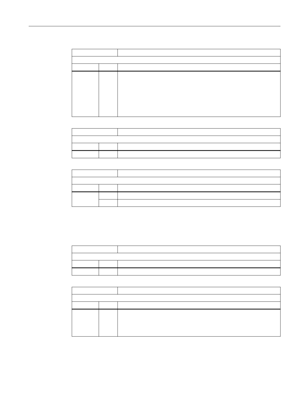
Velocities, setpoint/actual value systems, closed-loop control

5.4 Setpoint/actual-value system

MD30110

$MA_CTRLOUT_MODULE_NR

Setpoint assignment: Drive number / module number

System

Value

Meaning

The logical I/O address of the drive is assigned from MD13050 $MN_DRIVE_LOG-

IC_ADDRESS[ n ] via the drive number.

The drive number (x) results from the index (n) of MD13050:

x = n + 1

Note

The machine data is of no significance if the drive is simulated (MD30130

$MA_CTRLOUT_TYPE = 0).

MD30120

$MA_CTRLOUT_NR

Setpoint assignment: Setpoint output on drive module/module

System

Value

Meaning

Modular drive at PROFIBUS / PROFINET with PROFIdrive profile (default)

MD30130

$MA_CTRLOUT_TYPE

Setpoint output type

System

Value

Meaning

Simulation (operation without drive)

Setpoint output active

Encoder assignment

The following machine data is relevant for assigning the encoder information of the drive -

transferred in the PROFIdrive telegram - to the encoder inputs of the machine axis:

MD30210

$MA_ENC_SEGMENT_NR[ n ]

Actual value assignment, bus segment

System

Value

Meaning

PROFIBUS DP / PROFINET

MD30220

$MA_ENC_MODULE_NR[ n ]

Actual value assignment: Drive number/measuring circuit number

System

Value

Meaning

The logical I/O address of the drive is assigned from MD13050 $MN_DRIVE_LOG-

IC_ADDRESS[ n ] via the drive number.

The drive number (x) results from the index (n) of MD13050:

x = n + 1

Axes and spindles

Function Manual, 10/2020, 6FC5397-4GP40-0BA1

157

Velocities, setpoint/actual value systems, closed-loop control

5.4 Setpoint/actual-value system

MD30230

$MA_ENC_INPUT_NR[ n ]

Actual value assignment: Input on drive module/measuring circuit module

System

Value

Meaning

Number of the encoder interface within the PROFIdrive telegram

Examples

PROFIdrive telegram 103

x = 1 → 1st encoder interface (G1_ZSW, G1_XIST1, G1_XIST2)

x = 2 → 2nd encoder interface (G2_ZSW, G2_XIST1, G2_XIST2)

PROFIdrive telegram 118

x = 1 → 1st encoder interface (G2_ZSW, G2_XIST1, G2_XIST2)

x = 2 → 2nd encoder interface (G3_ZSW, G3_XIST1, G3_XIST2)

Note:

For SINAMICS S120:

- Encoder 1 (G1_...): Motor encoder

- Encoder 2 (G2_...): Direct measuring system

- Encoder 3 (G3_...): Additional measuring system

MD30240

$MA_ENC_TYPE[ n ]

Encoder type of actual value acquisition (actual position value)

System

Value

Meaning

Simulation (operation without encoder)

Incremental encoder

Absolute encoder

Note:

Corresponds to PROFIdrive parameter p979

Axes and spindles

158

Function Manual, 10/2020, 6FC5397-4GP40-0BA1

Velocities, setpoint/actual value systems, closed-loop control

5.4 Setpoint/actual-value system

MD30242

$MA_ENC_IS_INDEPENDENT[ n, axis ]

Encoder is independent

System

Value

Meaning

The encoder is not independent.

The encoder is independent.

If the actual-value corrections, which are made for the encoder selected for the

position control, are not to influence the actual value of the second encoder

defined in the same axis, then this should be declared as independent.

Actual value corrections are:

•

- Modulo treatment

•

- Reference point approach

•

- Measuring system alignment

•

- PRESET

Example: One axis, two encoders, the 2nd encoder is independent

MD30200 $MA_NUM_ENCS[ AX1 ] = 2

MD30242 $MA_ENC_IS_INDEPENDENT[ 0, AX1 ] = 0

MD30242 $MA_ENC_IS_INDEPENDENT[ 1, AX1 ] = 1

Selection, position measuring system 1 / 2: DB31.DBX1.5 / 1.6

If encoder 1 is selected for closed-loop position control, then the actual value

corrections are only performed on this encoder, as encoder 2 is independent.

If encoder 2 is selected for position control, then the actual value corrections are

performed on both encoders, as encoder 1 is not independent.

This means that the machine data only has an effect on the passive encoder of a

machine axis.

The passive encoder is dependent.

The actual encoder value is changed by the active encoder. In combination with

MD35102 $MA_REFP_SYNC_ENCS = 1, for reference point approach, the passive

encoder is aligned to the active encoder - but is NOT referenced.

In the referencing mode MD34200 $MA_ENC_REFP_MODE = 3 (distance-coded

reference marks) the passive encoder is automatically referenced with the next

traversing motion after passing the zero mark distance. This is done independent

of the actual operating mode setting.

The encoder is independent.

For modulo rotary axes, modulo actual value corrections are also performed in

the passive encoder.

Axes and spindles

Function Manual, 10/2020, 6FC5397-4GP40-0BA1

159

SINUMERIK 840D sl. Service - Functions. Manual (2018-2020) - page 5